Getting started with ROSAT All Sky Survey data#
Learning Goals#
By the end of this tutorial, you will be able to:
Fetch a catalog from Vizier and cross-match it with a catalog hosted by HEASARC.
Identify and fetch ROSAT All-Sky Survey (RASS) data relevant to a sample of sources.
Examine pregenerated RASS images.
Generate new RASS images with custom spatial binning and energy bands.
Acquire the ROSAT-PSPCC Redistribution Matrix File (RMF), extract RASS spectra, and generate Ancillary Response Files (ARFs) for a sample of sources; then fit models using PyXSPEC and extract results.
Introduction#
The ROSAT All Sky Survey (RASS) was, unsurprisingly, a survey that observed the entire sky using the ROSAT (standing for ‘Röntgensatellit’) X-ray mission. ROSAT launched in 1990 and was active until the beginning of 1999, when it was shut down after significant deterioration of the satellite’s navigational systems.
Three X-ray instruments could be moved into the focal plane of the single X-ray telescope mounted on the spacecraft (though they could not be used simultaneously):
High Resolution Imager (HRI) - A micro-channel plate (MCP) imager very similar to the one flown on the Einstein Observatory in 1978. High spatial resolution (~\(2^{\prime\prime}\)), but effectively no spectral resolution.
Position Sensitive Proportional Counter B (PSPCB) - One of a pair of proportional counters that could measure the position and energy of an incident photon using the charge produced when it was absorbed by the detector gas. Had moderate spatial resolution (~\(25^{\prime\prime}\)), low spectral resolution (~41% at 1 keV), and was sensitive in the 0.07–2.4 keV range.
Position Sensitive Proportional Counter C (PSPCC) - The second of a pair of proportional counters, PSPCC was the primary instrument, and was used to perform the ROSAT All-Sky Survey at the beginning of the mission. It was destroyed in 1991 after an error caused ROSAT to slew across the Sun.
ROSAT also had an extreme ultraviolet (XUV) imager called the Wide Field Camera (WFC), with a 5\(^{\circ}\) diameter field of view (FoV), a spatial resolution of ~\(2.3^{\prime}\), and was sensitive between 62–206 eV (~60–100 Å).
The ROSAT All-Sky Survey was taken using the ROSAT-PSPCC instrument, though it was left incomplete following the destruction of the instrument in 1991. Follow-up observations to fill in the gaps were performed using the PSPCB instrument much later in the mission’s life, but were taken in ‘pointed’ rather than ‘scanning’ mode, and as such are not included in the RASS archive. Instead, they are archived with all other pointed ROSAT observations and will not be used in this demonstration.
The effective angular resolution of RASS was worse than that of the PSPC instruments, at ~45\(^{\prime\prime}\), as the spacecraft was constantly slewing while taking the observations.
RASS’ data are organized into ‘skyfields’, each with their own sequence ID. Each skyfield represents a \(6.4^{\circ}\times6.4^{\circ}\) area of the sky, and is built from multiple slewing observations.
This tutorial will give you the skills required to start using RASS observations to measure X-ray properties of a set of sources. To demonstrate, we will be using a sample of over 700 M dwarf stars from the ‘CARMENES input catalogue of M dwarfs’ (Alonso-Floriano F. J. et al. 2015). We won’t be analyzing the entire dataset. However, there will still be a substantial number of sources to work with, which will give you an idea of how to use RASS data for large samples (one of the best use cases).
We also hope to make clear the limitations of what you can do with RASS data; ROSAT is one of the older X-ray missions and utilized less sophisticated instrumentation and optics than more modern observatories. That does impose restrictions on what we can reasonably expect to achieve, in terms of energy range coverage, sensitivity, and spectral/spatial resolution.
On the other hand, the ROSAT All-Sky Survey is still (as of early 2026), the only publicly available all-sky X-ray imaging dataset, with over 1.35e+5 sources in the ‘Second ROSAT all-sky survey’ source catalog (2RXS; Boller T. et al. 2016). The scientific potential of the RASS archive is still very great, and being able to directly analyze the data, rather than rely solely on catalogs, may help you with your own research interests.
Inputs#
The CARMENES input catalogue of M dwarfs (Alonso-Floriano F. J. et al. 2015).
Outputs#
Visualizations of pre-processed RASS images.
Newly generated RASS images.
Source/background region files and spectra.
Result table from fitting spectral models using PyXSPEC, and accompanying visualizations of spectra.
Runtime#
As of 12th March 2026, this notebook takes ~13 m to run to completion on Fornax using the ‘medium’ server with 16GB RAM/ 4 cores.
Imports#
import contextlib
import multiprocessing as mp
import os
from random import randint
from shutil import copyfile, rmtree
from typing import Tuple
from warnings import warn

import heasoftpy as hsp
import matplotlib.pyplot as plt
import numpy as np
import pandas as pd
import pyvo as vo
from astropy.coordinates import SkyCoord
from astropy.io import fits
from astropy.units import Quantity
from astropy.wcs import WCS
from astroquery.heasarc import Heasarc
from astroquery.vizier import Vizier
from matplotlib.ticker import FuncFormatter
from regions import CircleAnnulusSkyRegion, CircleSkyRegion, Regions, SkyRegion
from tqdm import tqdm
from xga.imagetools.misc import pix_deg_scale
from xga.products import EventList, ExpMap, Image, RateMap
/opt/envs/heasoft/lib/python3.12/site-packages/xga/utils.py:39: DeprecationWarning: The XGA 'find_all_wcs' function should be imported from imagetools.misc, in the future it will be removed from utils.
  warn(message, DeprecationWarning)
/opt/envs/heasoft/lib/python3.12/site-packages/xga/utils.py:619: UserWarning: SAS_DIR environment variable is not set, unable to verify SAS is present on system, as such all functions in xga.sas will not work.
  warn("SAS_DIR environment variable is not set, unable to verify SAS is present on system, as such "
/opt/envs/heasoft/lib/python3.12/site-packages/xga/__init__.py:6: UserWarning: This is the first time you've used XGA; to use most functionality you will need to configure /home/jovyan/.config/xga/xga.cfg to match your setup, though you can use product classes regardless.
  from .utils import xga_conf, CENSUS, OUTPUT, NUM_CORES, XGA_EXTRACT, BASE_XSPEC_SCRIPT, CROSS_ARF_XSPEC_SCRIPT, \
Global Setup#
Functions#
Constants#
Configuration#
1. Fetching the CARMENES M dwarf catalog and matching to a RASS catalog#
We stated in the introduction that we would use the CARMENES ‘input catalog of M dwarfs’ as the starting point for this demonstration. That way, we can show you how to approach RASS data analysis for a sample of sources.
To use the catalog, we’re going to need to acquire it from somewhere. In this case, that somewhere is the VizieR service (DOI:10.26093/cds/vizier), which we will access using the Astroquery Python module (Ginsburg et al. 2019).
Getting the CARMENES catalog from VizieR#
We have already imported the Vizier class from Astroquery, so we can now
set up an instance of it (with some non-default arguments) that can be used to fetch
our catalog of interest.
The row_limit=-1 argument tells Astroquery to return all rows from the catalog, and
the columns=["**", "_RAJ2000", "_DEJ2000"] tells it to also return every column (as
well as the VizieR-standard decimal degree RA and Dec values):
viz = Vizier(row_limit=-1, columns=["**", "_RAJ2000", "_DEJ2000"])
viz
<astroquery.vizier.core.VizierClass at 0x7e4b515f1a30>
We already know the ‘bibcode’ of the CARMENES catalog (J/A+A/577/A128), but if you
didn’t, you could search VizieR using the viz object we created.
By passing a list of keywords (every keyword must be associated with a catalog for
that catalog to be returned) to the find_catalogs() method, we find a few possible
matches. To narrow them down further, we can display the short description of each
returned catalog:
cat_search = viz.find_catalogs(["CARMENES", "input"])

# Return is an ordered dictionary, with bibcode keys and catalog object values
for cur_bibcode, cur_cat in cat_search.items():
    print(cur_bibcode, "-", cur_cat.description)
J/A+A/577/A128 - CARMENES input catalogue of M dwarfs. I (Alonso-Floriano+, 2015)
J/A+A/597/A47 - CARMENES input catalogue of M dwarfs II (Cortes-Contreras+ 2017)
J/A+A/614/A76 - CARMENES input catalogue of M dwarfs. III. (Jeffers+, 2018)
J/A+A/621/A126 - CARMENES input catalogue of M dwarfs. IV. (Diez Alonso+ 2019)
J/A+A/642/A115 - CARMENES input catalogue of M dwarfs. V. (Cifuentes+, 2020)
J/A+A/652/A116 - CARMENES time-resolved CaII H&K catalog (Perdelwitz+, 2021)
J/A+A/684/A9 - Rotation periods for 261 M dwarfs (Shan+, 2024)
J/A+A/692/A206 - CARMENES input cat. of M dwarfs VIII (Cortes-Contreras+, 2024)
J/A+A/693/A228 - CARMENES input catalogue of M dwarfs. IX. (Cifuentes+, 2025)
With the short descriptions shown above, you should be able to find the bibcode of the catalog you’re interested in.
Passing the bibcode of your chosen catalog to the get_catalogs() method presents
us with a TableList object that contains one entry per table included in the
catalog.
The CARMENES catalog we’re looking at contains two tables:
The first is the catalog of M dwarfs we’re going to use.
The second contains the literature references from which the catalog was compiled.
carm_samp = viz.get_catalogs("J/A+A/577/A128")
carm_samp
TableList with 2 tables:
	'0:J/A+A/577/A128/Mstars' with 40 column(s) and 753 row(s)
	'1:J/A+A/577/A128/refs' with 5 column(s) and 61 row(s)
We pull out the main catalog table, which is an Astropy Table object:
carm_cat = carm_samp[0]
carm_cat
| _RAJ2000 | _DEJ2000 | recno | No | Karmn | Name | Gl/GJ | RAJ2000 | DEJ2000 | Jmag | Date | Nexp | texp | Nexp2 | texp2 | PC1 | TiO2 | TiO5 | VO | Col-M | CaH2 | CaH3 | zeta | pEWa | e_pEWa | E_pEWa | SpTl | r_SpTl | l_SpTb | SpTb | l_SpTc | SpTc | SpT2 | SpT5 | SpTP | SpTR | SpTC | l_SpT | SpT | Simbad |
|---|---|---|---|---|---|---|---|---|---|---|---|---|---|---|---|---|---|---|---|---|---|---|---|---|---|---|---|---|---|---|---|---|---|---|---|---|---|---|---|
| deg | deg | mag | s | s | 0.1 nm | 0.1 nm | 0.1 nm | ||||||||||||||||||||||||||||||||
| float64 | float64 | int32 | int16 | str13 | str23 | str8 | str11 | str11 | float32 | str10 | uint8 | float32 | uint8 | int16 | float32 | float32 | float32 | float32 | float32 | float32 | float32 | float32 | float32 | float32 | float32 | str15 | str16 | str2 | float32 | str2 | float32 | float32 | float32 | float32 | float32 | float32 | str1 | str7 | str6 |
| 1.6633333 | -7.0931389 | 1 | 1 | J00066-070AB | 2MASS J00063925-0705354 | 00 06 39.20 | -07 05 35.3 | 9.83 | 2012-08-04 | 1 | 1000.0 | -- | -- | 1.269 | 0.492 | 0.317 | 1.148 | 1.778 | 0.404 | 0.654 | 0.973 | -2.3 | 0.5 | 0.3 | M3.5V+m4.5: | Reid07,Jan12 | 4.5 | 4.5 | 4.5 | 4.5 | 4.0 | 4.5 | 4.5 | M4.5V | Simbad | ||||
| 1.9275000 | 60.3817500 | 2 | 2 | J00077+603AB | G 217-032 | 00 07 42.60 | +60 22 54.3 | 8.91 | 2012-09-24 | 1 | 600.0 | -- | -- | 1.198 | 0.532 | 0.369 | 1.111 | 1.405 | 0.408 | 0.631 | 0.883 | -6.7 | 0.4 | 0.3 | M4.5V | Lep13 | 4.0 | 4.0 | 4.5 | 4.0 | 3.5 | 4.0 | 3.5 | M4.0V | Simbad | ||||
| 2.8825833 | 59.1444444 | 3 | 3 | J00115+591 | LSR J0011+5908 | 00 11 31.82 | +59 08 40.0 | 9.95 | 2012-01-11 | 2 | 700.0 | -- | -- | 1.511 | 0.378 | 0.202 | 1.222 | 2.902 | 0.281 | 0.564 | 0.970 | -1.6 | 0.4 | 0.2 | M5.5V | Lep03 | 6.0 | 6.0 | 5.5 | 6.0 | 5.5 | 5.5 | 5.5 | M5.5V | Simbad | ||||
| 2.9709583 | 22.9846389 | 4 | 4 | J00118+229 | LP 348-40 | 00 11 53.03 | +22 59 04.7 | 8.86 | 2011-12-07 | 1 | 250.0 | -- | -- | 1.215 | 0.606 | 0.405 | 1.090 | 1.404 | 0.492 | 0.751 | 1.052 | -0.5 | 0.2 | 0.2 | M3.5V | Reid04 | 3.5 | 3.5 | 3.5 | 3.5 | 4.0 | 4.0 | 3.5 | M3.5V | Simbad | ||||
| 2.9855833 | 33.0549444 | 5 | 5 | J00119+330 | G 130-053 | 00 11 56.54 | +33 03 17.8 | 9.07 | 2011-12-07 | 1 | 220.0 | -- | -- | 1.167 | 0.634 | 0.427 | 1.072 | 1.293 | 0.503 | 0.748 | 1.023 | -0.3 | 0.2 | 0.1 | M3.5V | Giz97 | 3.5 | 3.0 | 3.5 | 3.5 | 3.5 | 3.5 | 3.5 | M3.5V | Simbad | ||||
| 3.0558750 | 30.4789722 | 6 | 6 | J00122+304 | 1RXS J001213.6+302906 | 00 12 13.41 | +30 28 44.3 | 10.24 | 2011-11-12 | 1 | 600.0 | -- | -- | 1.296 | 0.497 | 0.354 | 1.154 | 1.755 | 0.427 | 0.685 | 0.972 | -8.7 | 0.5 | 0.4 | M5.0V | Abe14 | 4.5 | 4.5 | 4.5 | 4.0 | 4.5 | 5.0 | 4.5 | M4.5V | Simbad | ||||
| 3.3313333 | 27.5586389 | 7 | 7 | J00133+275 | [ACM2014] J0013+2733 | 00 13 19.52 | +27 33 31.1 | 10.43 | 2011-11-12 | 1 | 900.0 | -- | -- | 1.296 | 0.512 | 0.339 | 1.144 | 1.805 | 0.425 | 0.686 | 0.994 | -4.0 | 0.4 | 0.2 | M4.5V | Abe14 | 4.5 | 4.5 | 4.5 | 4.5 | 4.5 | 4.5 | 4.5 | M4.5V | Simbad | ||||
| 3.4112917 | 80.6657778 | 8 | 8 | J00136+806 | G 242-048 | 3014 A | 00 13 38.71 | +80 39 56.8 | 7.76 | 2012-09-01 | 1 | 300.0 | -- | -- | 1.027 | 0.770 | 0.601 | 1.012 | 0.901 | 0.644 | 0.812 | 1.002 | 0.0 | 0.2 | 0.2 | M1.5V | PMSU | 1.5 | 1.5 | 1.5 | 1.5 | 1.5 | 1.5 | 1.5 | M1.5V | Simbad | |||
| 3.6506667 | 20.2066944 | 9 | 9 | J00146+202 | chi Peg | 00 14 36.16 | +20 12 24.1 | 1.76 | 2012-01-11 | 1 | 1.0 | -- | -- | 0.955 | 0.729 | 0.520 | 1.005 | 0.643 | 0.839 | 0.946 | 2.754 | 0.8 | 0.1 | 0.1 | M2III | Gar89,Kir91 | -- | -- | -- | -- | -- | -- | -- | MIII | Simbad | ||||
| ... | ... | ... | ... | ... | ... | ... | ... | ... | ... | ... | ... | ... | ... | ... | ... | ... | ... | ... | ... | ... | ... | ... | ... | ... | ... | ... | ... | ... | ... | ... | ... | ... | ... | ... | ... | ... | ... | ... | ... |
| 355.5921250 | 34.9743611 | 745 | 745 | J23423+349 | PM I23423+3458 | 23 42 22.11 | +34 58 27.7 | 9.32 | 2012-01-04 | 1 | 350.0 | -- | -- | 1.215 | 0.591 | 0.383 | 1.094 | 1.447 | 0.467 | 0.732 | 1.029 | -0.6 | 0.4 | 0.2 | 4.0 | 4.0 | 4.0 | 4.0 | 4.0 | 4.0 | 3.5 | M4.0V | Simbad | ||||||
| 355.6395833 | 39.2398056 | 746 | 746 | J23425+392 | LP 291-007 | 23 42 33.50 | +39 14 23.3 | 9.64 | 2012-01-09 | 1 | 1000.0 | -- | -- | 0.928 | 0.904 | 0.823 | 0.982 | 0.739 | 0.875 | 0.921 | 1.054 | -1.6 | 0.3 | 0.4 | 0.0 | 0.0 | -0.5 | -0.5 | 0.0 | 0.0 | 0.0 | M0.0V | Simbad | ||||||
| 355.9712500 | 61.0376944 | 747 | 747 | J23438+610 | G 217-018 | 23 43 53.10 | +61 02 15.7 | 9.39 | 2012-01-04 | 1 | 500.0 | -- | -- | 1.110 | 0.641 | 0.434 | 1.059 | 1.176 | 0.492 | 0.731 | 0.974 | 0.0 | 0.4 | 0.4 | k: | Simbad | 3.0 | 3.0 | 3.5 | 3.5 | 2.5 | 3.0 | 3.0 | M3.0V | Simbad | ||||
| 357.2595833 | -8.4085833 | 748 | 748 | J23490-086 | G 273-144 | 23 49 02.30 | -08 24 30.9 | 9.50 | 2012-08-02 | 1 | 272.0 | -- | -- | 1.054 | 0.737 | 0.534 | 1.029 | 0.999 | 0.563 | 0.775 | 0.947 | 0.0 | 0.4 | 0.4 | M2.5V | Reid04 | 2.0 | 2.0 | 2.0 | 2.5 | 2.0 | 2.0 | 2.0 | M2.0V | Simbad | ||||
| 358.9800000 | -13.3566111 | 749 | 749 | J23559-133 | NLTT 58441 | 23 55 55.20 | -13 21 23.8 | 9.26 | 2012-09-02 | 1 | 250.0 | -- | -- | 1.184 | 0.568 | 0.405 | 1.094 | 1.331 | 0.472 | 0.700 | 0.959 | -4.2 | 0.4 | 0.5 | M3.0V | Sch05 | 3.5 | 3.5 | 4.0 | 3.5 | 3.5 | 4.0 | 3.5 | M3.5V | Simbad | ||||
| 359.0012083 | 15.0280278 | 750 | 750 | J23560+150 | LP 523-078 | 23 56 00.29 | +15 01 40.9 | 9.38 | 2011-12-07 | 1 | 250.0 | -- | -- | 1.102 | 0.709 | 0.517 | 1.040 | 1.110 | 0.560 | 0.783 | 0.990 | 0.0 | 0.4 | 0.4 | 2.5 | 2.5 | 2.5 | 2.5 | 2.5 | 2.5 | 2.5 | M2.5V | Simbad | ||||||
| 359.2295833 | 23.0840833 | 751 | 751 | J23569+230 | G 129-045 | 23 56 55.10 | +23 05 02.7 | 9.15 | 2011-12-07 | 1 | 300.0 | -- | -- | 1.012 | 0.801 | 0.640 | 1.007 | 0.914 | 0.680 | 0.848 | 1.045 | 0.0 | 0.4 | 0.4 | K7V | Ste86 | 1.5 | 1.0 | 1.5 | 1.5 | 1.5 | 1.0 | 1.5 | M1.5V | Simbad | ||||
| 359.6258750 | 24.2013333 | 752 | 752 | J23585+242 | G 131-006 | 23 58 30.21 | +24 12 04.8 | 9.13 | 2012-09-04 | 1 | 90.0 | -- | -- | 0.898 | 0.921 | 0.836 | 0.977 | 0.677 | 0.905 | 0.931 | 1.105 | 0.5 | 0.2 | 0.3 | K7V | Lee84 | -1.0 | -1.0 | -1.0 | -1.0 | -1.0 | -0.5 | -0.5 | K7V | Simbad | ||||
| 359.7517500 | 20.8607778 | 753 | 753 | J23590+208 | G 129-051 | 23 59 00.42 | +20 51 38.8 | 9.07 | 2011-12-07 | 1 | 180.0 | -- | -- | 1.111 | 0.668 | 0.469 | 1.059 | 1.097 | 0.561 | 0.785 | 1.095 | 0.0 | 0.4 | 0.4 | 2.5 | 2.0 | 3.0 | 3.0 | 2.5 | 3.0 | 2.5 | M2.5V | Simbad |
Setting up a connection to the HEASARC TAP service#
So, we have the catalog of M dwarfs that we want to examine using the RASS data archive. At this point we could just feed the whole set of stars into the RASS analyses we perform later in this tutorial.
However, to simplify this demonstration, we would rather deal only with sources that have been detected in the ROSAT All-Sky Survey. To that end, we will perform a simple spatial cross-match between the CARMENES catalog and the 2RXS (Boller T. et al. 2016) catalog of RASS sources.
We will use the HEASARC Table Access Protocol (TAP) service to perform the cross-match, uploading the CARMENES table we just retrieved.
In order for us to be able to do that, we need to set up a connection to the HEASARC TAP service. Here we use the PyVO Python module to search for the right service:
tap_services = vo.regsearch(servicetype="tap", keywords=["heasarc"])
tap_services
<DALResultsTable length=1>
              ivoid                    res_type     ... cap_descriptions
                                                    ...
              object                    object      ...      object
--------------------------------- ----------------- ... ----------------
ivo://nasa.heasarc/services/xamin vs:catalogservice ...
We can extract the first entry from that search return, and we have our connection!
heasarc_vo = tap_services[0]
Writing a query to match CARMENES to 2RXS#
Now we have a connection to the HEASARC TAP service, we will be able to upload our CARMENES table and perform a simple cross-match.
All that’s left is to write and submit an Astronomical Data Query Language (ADQL) query (almost a tautology) that tells the HEASARC TAP service to try and identify a 2RXS entry within a search radius of each CARMENES M dwarf.
We already know the HEASARC name for the 2RXS catalog (which we store in a variable below). However, if you want to match to a different catalog that you don’t already know the HEASARC name for you might want to look at the ‘Find specific HEASARC catalogs using Python demonstration.
heasarc_cat_name = "rass2rxs"
We select a search radius of 8\(^{\prime\prime}\), though you should consider your own choice carefully as it will depend on your science goals and the type of objects you want to look at:
MATCH_RADIUS = Quantity(8, "arcsec")
Finally, we write the query itself. As ADQL queries go, it’s fairly simple; the only matching (and filtering) criteria we apply is that a 2RXS source must be within the search radius of a CARMENES source to be considered a match.
It’s worth noting that we will be able to run this query on all the CARMENES sources at once, rather than having to run it separately for every entry.
Breaking down the query:
SELECT *will return all columns from both tables.FROM {hcn} as rasscatwill ‘load’ the HEASARC catalog with the alias ‘rasscat’ ({hcn} will be replaced by ‘rass2rxs’ in this case).FROM ... tap_upload.carmenes as carmwill ‘load’ the table we upload (see the query submission subsection) with the alias ‘carm’.WHERE contains(point('ICRS',cat.ra,cat.dec), circle('ICRS',carm.{cra},carm.{cdec},{md}))=1will require that a 2RXS coordinate (cat.raandcat.dec) be within the search radius of a CARMENES coordinate (carm.{cra}andcarm.{cdec}) to be considered a match.
query = (
    "SELECT * "
    "FROM {hcn} as rasscat, tap_upload.carmenes as carm "
    "WHERE "
    "contains(point('ICRS',rasscat.ra,rasscat.dec), "
    "circle('ICRS',carm.{cra},carm.{cdec},{md}))=1".format(
        md=MATCH_RADIUS.to("deg").value.round(4),
        cra="_RAJ2000",
        cdec="_DEJ2000",
        hcn=heasarc_cat_name,
    )
)

query
"SELECT * FROM rass2rxs as rasscat, tap_upload.carmenes as carm WHERE contains(point('ICRS',rasscat.ra,rasscat.dec), circle('ICRS',carm._RAJ2000,carm._DEJ2000,0.0022))=1"
Preparing the CARMENES catalog for upload#
Actually, writing the query wasn’t really the last thing we needed to do. Before we upload the CARMENES table and submit the matching query we have to make some adjustments to the CARMENES catalog.
These adjustments are necessary to avoid errors when using the HEASARC TAP service to run the matching query. Firstly, the HEASARC TAP service will change all column names to their lowercase equivalents. So, if there are any columns that are identically named, apart from the case of some letters, we have to rename them:
carm_cat.rename_column("e_pEWa", "pEWa_errmi")
carm_cat.rename_column("E_pEWa", "pEWa_errpl")

carm_cat.rename_column("SpTC", "SpTColor")
Additionally, if you include RA and Dec columns that are in sexagesimal format (as opposed to decimal degrees), you may encounter an error since the distance-calculation function does not work on string data types. As such, and because the author of this tutorial is biased against sexagesimal coordinates, we will just remove those columns:
carm_cat.remove_columns(["RAJ2000", "DEJ2000"])
Finally, we add a new column with a clean identifying name for each CARMENES source, based on the ‘No’ column containing the CARMENES unique entry number. When we start generating data products, it’s good to know you have IDs to include in file and directory names that don’t include special characters or spaces.
We note that the ‘Karmn’ column included in the CARMENES catalog would be another good candidate for this purpose.
carm_cat.add_column(
    ["CARMENES-" + str(carm_id) for carm_id in carm_cat["No"]], name="id_name"
)
Submitting the query to the HEASARC TAP service#
All the pieces have come together, and we can run the CARMENES-2RXS cross-match query
by passing it to the service.run_sync(...) method of the HEASARC TAP service
connection we retrieved earlier.
The CARMENES catalog can be passed straight into the uploads argument as it is an
Astropy Table object. Note that the key of the dictionary passed to the uploads
argument must match the name of the table in the query
defined previously.
carm_2rxs_match = heasarc_vo.service.run_sync(query, uploads={"carmenes": carm_cat})
We can then convert the return to an Astropy Table and visualize it:
carm_2rxs_match = carm_2rxs_match.to_table()
carm_2rxs_match
| rasscat___row | rasscat_entry_number | rasscat_name | rasscat_skyfield_number | rasscat_skyfield_source_number | rasscat_detection_likelihood | rasscat_counts | rasscat_counts_error | rasscat_count_rate | rasscat_count_rate_error | rasscat_exposure | rasscat_ra | rasscat_dec | rasscat_lii | rasscat_bii | rasscat_lambda | rasscat_beta | rasscat_source_extent | rasscat_source_extent_error | rasscat_source_extent_prob | rasscat_hardness_ratio_1 | rasscat_hardness_ratio_1_error | rasscat_hardness_ratio_2 | rasscat_hardness_ratio_2_error | rasscat_unique_flag | rasscat_extended_region_flag | rasscat_nearby_src_det_flag | rasscat_source_quality_flag | rasscat_max_amplitude | rasscat_mean_count_rate | rasscat_mean_count_rate_error | rasscat_lc_counts | rasscat_min_count_rate | rasscat_min_count_rate_error | rasscat_max_count_rate | rasscat_max_count_rate_error | rasscat_lc_chi2 | rasscat_excess_variance | rasscat_excess_variance_error | rasscat_excess_variance_sigma | rasscat_nh_gal | rasscat_plaw_nh | rasscat_plaw_nh_error | rasscat_plaw_norm | rasscat_plaw_norm_error | rasscat_plaw_photon_index | rasscat_plaw_photon_index_error | rasscat_plaw_count_rate | rasscat_plaw_flux | rasscat_plaw_chi2_reduced | rasscat_plaw_chi2 | rasscat_plaw_number_data_pts | rasscat_plaw_dof | rasscat_mekal_nh | rasscat_mekal_nh_error | rasscat_mekal_norm | rasscat_mekal_norm_error | rasscat_mekal_temperature | rasscat_mekal_temperature_error | rasscat_mekal_count_rate | rasscat_mekal_flux | rasscat_mekal_chi2_reduced | rasscat_mekal_chi2 | rasscat_mekal_number_data_pts | rasscat_mekal_dof | rasscat_bb_nh | rasscat_bb_nh_error | rasscat_bb_norm | rasscat_bb_norm_error | rasscat_bb_temperature | rasscat_bb_temperature_error | rasscat_bb_count_rate | rasscat_bb_flux | rasscat_bb_chi2_reduced | rasscat_bb_chi2 | rasscat_bb_number_data_pts | rasscat_bb_dof | rasscat_x_pixel | rasscat_x_pixel_error | rasscat_y_pixel | rasscat_y_pixel_error | rasscat_x_sky_pixel | rasscat_y_sky_pixel | rasscat_extraction_radius | rasscat_extraction_radius_frac | rasscat_total_photons | rasscat_bkg_in_extr_reg | rasscat_vignetting_factor | rasscat_remarks | rasscat_band_a_tot_counts | rasscat_band_b_tot_counts | rasscat_band_c_tot_counts | rasscat_band_d_tot_counts | rasscat_band_a_bkg_counts | rasscat_band_b_bkg_counts | rasscat_band_c_bkg_counts | rasscat_band_d_bkg_counts | rasscat_remaining_bkg_area | rasscat_band_a_counts | rasscat_band_b_counts | rasscat_band_c_counts | rasscat_band_d_counts | rasscat_xmmsl1_number_ctrprts | rasscat_xmmsl1_nearest | rasscat_xmmsl1_separation | rasscat_xmmsl1_name | rasscat_xmmsl1_ra | rasscat_xmmsl1_dec | rasscat_xmmsl1_bb_count_rate | rasscat_xmmsl1_bb_count_rate_err | rasscat_xmmsl1_sb_count_rate | rasscat_xmmsl1_sb_count_rate_err | rasscat_threexmm_number_ctrprts | rasscat_threexmm_nearest | rasscat_threexmm_separation | rasscat_threexmm_name | rasscat_threexmm_ra | rasscat_threexmm_dec | rasscat_threexmm_count_rate | rasscat_threexmm_count_rate_err | rasscat_threexmm_flux | rasscat_threexmm_flux_error | rasscat_tworxp_number_ctrprts | rasscat_tworxp_nearest | rasscat_tworxp_separation | rasscat_tworxp_name | rasscat_tworxp_ra | rasscat_tworxp_dec | rasscat_tworxp_count_rate | rasscat_tworxp_count_rate_error | rasscat_tworxp_exposure | rasscat_tworxp_obsid | rasscat_onerxs_number_ctrprts | rasscat_onerxs_nearest | rasscat_onerxs_separation | rasscat_onerxs_name | rasscat_onerxs_ra | rasscat_onerxs_dec | rasscat_onerxs_count_rate | rasscat_onerxs_count_rate_error | rasscat_onerxs_counts | rasscat_onerxs_counts_error | rasscat_onerxs_det_likelihood | rasscat_onerxs_exposure | rasscat_onerxs_hr_1 | rasscat_onerxs_hr_1_error | rasscat_onerxs_hr_2 | rasscat_onerxs_hr_2_error | rasscat_veron_number_ctrprts | rasscat_veron_nearest | rasscat_veron_separation | rasscat_veron_name | rasscat_veron_type | rasscat_veron_vmag | rasscat_veron_redshift | rasscat_veron_source_number | rasscat_veron_ra | rasscat_veron_dec | rasscat_tycho2_number_ctrprts | rasscat_tycho2_nearest | rasscat_tycho2_separation | rasscat_tycho2_ra | rasscat_tycho2_dec | rasscat_tycho2_source_number | rasscat_tycho2_vmag | rasscat_tycho2_bmag | rasscat_tycho2_tyc1_number | rasscat_tycho2_tyc2_number | rasscat_tycho2_tyc3_number | rasscat_bsc_number_ctrprts | rasscat_bsc_nearest | rasscat_bsc_separation | rasscat_bsc_ra | rasscat_bsc_dec | rasscat_bsc_vmag | rasscat_bsc_spect_type | rasscat_bsc_source_number | rasscat_hd_source_number | rasscat_hmxb_number_ctrprts | rasscat_hmxb_nearest | rasscat_hmxb_separation | rasscat_hmxb_name | rasscat_hmxb_alt_name | rasscat_hmxb_ra | rasscat_hmxb_dec | rasscat_hmxb_vmag | rasscat_lmxb_number_ctrprts | rasscat_lmxb_nearest | rasscat_lmxb_separation | rasscat_lmxb_name | rasscat_lmxb_alt_name | rasscat_lmxb_ra | rasscat_lmxb_dec | rasscat_lmxb_vmag | rasscat_atnf_number_ctrprts | rasscat_atnf_nearest | rasscat_atnf_separation | rasscat_atnf_name | rasscat_atnf_ra | rasscat_atnf_dec | rasscat_atnf_pulsar_type | rasscat_atnf_pulse_period | rasscat_fuhr_number_ctrprts | rasscat_fuhr_nearest | rasscat_fuhr_separation | rasscat_fuhr_name | rasscat_fuhr_ra | rasscat_fuhr_dec | rasscat_fuhr_source_number | rasscat_onesxps_number_ctrprts | rasscat_onesxps_nearest | rasscat_onesxps_separation | rasscat_onesxps_ra | rasscat_onesxps_dec | rasscat_onesxps_exposure | rasscat_onesxps_det_flag | rasscat_onesxps_total_det_flag | rasscat_onesxps_soft_det_flag | rasscat_onesxps_medium_det_flag | rasscat_onesxps_hard_det_flag | rasscat_onesxps_source_number | rasscat_onesxps_count_rate | rasscat_onesxps_count_rate_error | rasscat_onerxh_number_ctrprts | rasscat_onerxh_nearest | rasscat_onerxh_separation | rasscat_onerxh_name | rasscat_onerxh_ra | rasscat_onerxh_dec | rasscat_onerxh_count_rate | rasscat_onerxh_count_rate_error | rasscat_onerxh_exposure | rasscat_onerxh_snr | rasscat_flem_number_ctrprts | rasscat_flem_nearest | rasscat_flem_separation | rasscat_flem_name | rasscat_flem_ra | rasscat_flem_dec | rasscat_flem_type | rasscat_flem_wfc_detection_flag | rasscat_flem_count_rate | rasscat_flem_count_rate_error | rasscat_wdcat_number_ctrprts | rasscat_wdcat_nearest | rasscat_wdcat_separation | rasscat_wdcat_name | rasscat_wdcat_ra | rasscat_wdcat_dec | rasscat_wdcat_vmag | rasscat_wdcat_vsphot | rasscat_sdss_number_ctrprts | rasscat_sdss_nearest | rasscat_sdss_separation | rasscat_sdss_name | rasscat_sdss_ra | rasscat_sdss_dec | rasscat_sdss_lambda | rasscat_sdss_beta | rasscat_tworxs_number_ctrprts | rasscat_tworxs_nearest_src_num | rasscat_tworxs_nearest_src_index | rasscat_tworxs_separation | rasscat_tworxs_skyfield_number | rasscat_tworxs_skyfield_src_num | rasscat_tworxs_det_likelihood | rasscat_tworxs_count_rate | rasscat_tworxs_ra | rasscat_tworxs_dec | rasscat_tworxs_subfield_det_cell | rasscat_tworxs_nearby_flag | rasscat_tworxs_selected_bkg | rasscat_tworxs_x_pixel_sky_bkg1 | rasscat_tworxs_y_pixel_sky_bkg1 | rasscat_tworxs_x_pixel_sky_bkg2 | rasscat_tworxs_y_pixel_sky_bkg2 | rasscat_onerxs_bkg_count_rate | rasscat_tworxs_bkg_count_rate | rasscat_var_flag | rasscat_count_rate_6s | rasscat_count_rate_6s_error | rasscat_excess_var_6s | rasscat_excess_var_6s_error | rasscat_number_pts_in_lc | rasscat_number_pts_lessthan_6s | rasscat_number_pts_lessthan_1s | rasscat_number_pts_gtrthan_6s | rasscat_min_count_rate_6s | rasscat_max_count_rate_6s | rasscat_min_count_rate_6s_error | rasscat_max_count_rate_6s_error | rasscat_counts_notused_6 | rasscat_excess_var_lessthan_6 | rasscat_sum_count_rate_sigma | rasscat_spect_plot_flag | rasscat_lc_plot_flag | rasscat_clock_time | rasscat_clock_end_time | rasscat_time | rasscat_end_time | rasscat___x_ra_dec | rasscat___y_ra_dec | rasscat___z_ra_dec | carm__raj2000 | carm__dej2000 | carm_recno | carm_no | carm_karmn | carm_name | carm_gl_gj | carm_jmag | carm_date | carm_nexp | carm_texp | carm_nexp2 | carm_texp2 | carm_pc1 | carm_tio2 | carm_tio5 | carm_vo | carm_col_m | carm_cah2 | carm_cah3 | carm_zeta | carm_pewa | carm_pewa_errmi | carm_pewa_errpl | carm_sptl | carm_r_sptl | carm_l_sptb | carm_sptb | carm_l_sptc | carm_sptc | carm_spt2 | carm_spt5 | carm_sptp | carm_sptr | carm_sptcolor | carm_l_spt | carm_spt | carm_simbad | carm_id_name |
|---|---|---|---|---|---|---|---|---|---|---|---|---|---|---|---|---|---|---|---|---|---|---|---|---|---|---|---|---|---|---|---|---|---|---|---|---|---|---|---|---|---|---|---|---|---|---|---|---|---|---|---|---|---|---|---|---|---|---|---|---|---|---|---|---|---|---|---|---|---|---|---|---|---|---|---|---|---|---|---|---|---|---|---|---|---|---|---|---|---|---|---|---|---|---|---|---|---|---|---|---|---|---|---|---|---|---|---|---|---|---|---|---|---|---|---|---|---|---|---|---|---|---|---|---|---|---|---|---|---|---|---|---|---|---|---|---|---|---|---|---|---|---|---|---|---|---|---|---|---|---|---|---|---|---|---|---|---|---|---|---|---|---|---|---|---|---|---|---|---|---|---|---|---|---|---|---|---|---|---|---|---|---|---|---|---|---|---|---|---|---|---|---|---|---|---|---|---|---|---|---|---|---|---|---|---|---|---|---|---|---|---|---|---|---|---|---|---|---|---|---|---|---|---|---|---|---|---|---|---|---|---|---|---|---|---|---|---|---|---|---|---|---|---|---|---|---|---|---|---|---|---|---|---|---|---|---|---|---|---|---|---|---|---|---|---|---|---|---|---|---|---|---|---|---|---|---|---|---|---|---|---|---|---|---|---|---|---|---|---|---|---|---|---|---|---|---|---|---|---|---|---|---|---|---|---|---|---|---|---|---|---|---|---|---|---|---|---|---|---|---|---|---|---|---|---|---|---|---|---|---|---|---|---|---|---|---|---|---|---|---|---|
| ct | ct | ct / s | ct / s | s | deg | deg | deg | deg | deg | deg | pix | pix | ct / s | ct / s | ct | ct / s | ct / s | ct / s | ct / s | sigma | 1 / cm2 | 1 / cm2 | 1 / cm2 | ct / s | erg/s/cm^2 | 1 / cm2 | 1 / cm2 | ct / s | erg/s/cm^2 | 1 / cm2 | 1 / cm2 | ct / s | erg/s/cm^2 | pix | pix | pix | pix | pix | pix | pix | 1 / pix | ct | ct | ct | ct | ct | ct | ct | ct | arcmin2 | ct | ct | ct | ct | arcsec | deg | deg | ct / s | ct / s | c / s | c / s | arcsec | deg | deg | ct / s | ct / s | erg/s/cm^2 | erg/s/cm^2 | arcsec | deg | deg | ct / s | ct / s | s | arcsec | deg | deg | ct / s | ct / s | s | arcsec | mag | deg | deg | arcsec | deg | deg | mag | mag | arcsec | deg | deg | mag | arcsec | deg | deg | mag | arcsec | deg | deg | mag | arcsec | deg | deg | s | arcsec | deg | deg | arcsec | deg | deg | s | ct / s | ct / s | arcsec | deg | deg | ct / s | ct / s | s | arcsec | deg | deg | ct / s | ct / s | arcsec | deg | deg | mag | mag | arcsec | deg | deg | deg | deg | arcsec | ct / s | deg | deg | pix | pix | pix | pix | ct/s/arcmin^2 | ct/s/arcmin^2 | ct / s | ct / s | ct / s | ct / s | ct / s | ct / s | s | s | d | d | deg | deg | mag | s | s | 0.1 nm | 0.1 nm | 0.1 nm | ||||||||||||||||||||||||||||||||||||||||||||||||||||||||||||||||||||||||||||||||||||||||||||||||||||||||||||||||||||||||||||||||||||||||||||||||||||||||||||||||||||||||||||||||||
| int32 | int32 | object | int32 | int16 | float64 | float64 | float64 | float64 | float64 | float64 | float64 | float64 | float64 | float64 | float64 | float64 | float64 | float64 | float64 | float64 | float64 | float64 | float64 | int16 | int16 | int16 | int16 | float64 | float64 | float64 | float64 | float64 | float64 | float64 | float64 | float64 | float64 | float64 | float64 | float64 | float64 | float64 | float64 | float64 | float64 | float64 | float64 | float64 | float64 | float64 | int16 | int16 | float64 | float64 | float64 | float64 | float64 | float64 | float64 | float64 | float64 | float64 | int16 | int16 | float64 | float64 | float64 | float64 | float64 | float64 | float64 | float64 | float64 | float64 | int16 | int16 | float64 | float64 | float64 | float64 | float64 | float64 | int16 | float64 | int16 | float64 | float64 | object | float64 | float64 | float64 | float64 | float64 | float64 | float64 | float64 | float64 | float64 | float64 | float64 | float64 | int16 | int32 | float64 | object | float64 | float64 | float64 | float64 | float64 | float64 | int16 | int32 | float64 | object | float64 | float64 | float64 | float64 | float64 | float64 | int16 | int32 | float64 | object | float64 | float64 | float64 | float64 | int32 | object | int16 | int32 | float64 | object | float64 | float64 | float64 | float64 | float64 | float64 | int16 | int32 | float64 | float64 | float64 | float64 | int16 | int32 | float64 | object | object | float64 | float64 | int32 | float64 | float64 | int16 | int32 | float64 | float64 | float64 | int32 | float64 | float64 | int16 | int32 | int16 | int16 | int16 | float64 | float64 | float64 | float64 | object | int16 | int32 | int16 | int16 | float64 | object | object | float64 | float64 | float64 | int16 | int16 | float64 | object | object | float64 | float64 | float64 | int16 | int16 | float64 | object | float64 | float64 | object | object | int16 | int16 | float64 | object | float64 | float64 | object | int16 | int32 | float64 | float64 | float64 | int32 | int16 | int16 | int16 | int16 | int16 | int32 | float64 | float64 | int16 | int32 | float64 | object | float64 | float64 | float64 | float64 | int32 | float64 | int16 | int16 | float64 | object | float64 | float64 | object | object | float64 | float64 | int16 | int32 | float64 | object | float64 | float64 | float64 | float64 | int16 | int16 | float64 | object | float64 | float64 | float64 | float64 | int16 | int32 | int32 | float64 | int32 | int16 | float64 | float64 | float64 | float64 | int16 | int16 | int16 | float64 | float64 | float64 | float64 | float64 | float64 | int16 | float64 | float64 | float64 | float64 | int16 | int16 | int16 | int16 | float64 | float64 | float64 | float64 | float64 | float64 | float64 | int16 | int16 | float64 | float64 | float64 | float64 | float64 | float64 | float64 | float64 | float64 | int32 | int16 | object | object | object | float32 | object | int32 | float32 | int32 | int16 | float32 | float32 | float32 | float32 | float32 | float32 | float32 | float32 | float32 | float32 | float32 | object | object | object | float32 | object | float32 | float32 | float32 | float32 | float32 | float32 | object | object | object | object |
| 9241 | 9241 | 2RXS J000742.3+602250 | 930601 | 119 | 194.80 | 100.20 | 10.709172 | 0.1877 | 0.0201 | 533.72 | 1.92634 | 60.38077 | 117.54983 | -2.03318 | 36.16387 | 52.27769 | 0.363 | 0.287 | 2.37 | -0.444 | 0.079 | 0.045 | 0.169 | 5 | 1 | 0 | 0 | 0.1592 | 0.18298 | 0.10279 | 158.51 | 0.02817 | 0.06030 | 0.35723 | 0.10958 | 0.055 | 0.00345341 | 0.151196 | 0.022841 | 5.79e+21 | 1.96e+19 | 8.443e+19 | 0.0003209 | 0.0001265 | -1.8600 | 0.6094 | 0.203300 | 1.515e-12 | 0.9388 | 8.4490 | 12 | 9 | 5.128e+21 | 7.815e+22 | 0.0009433 | 0.001871 | 0.497500 | 9.717 | 0.058600 | 0.000000 | 7.387 | 66.48 | 12 | 9 | 1e+18 | 1.062e+20 | 0.002126 | 0.001458 | 0.142900 | 0.02485 | 0.175600 | 1.297e-12 | 1.98 | 17.82 | 12 | 9 | 395.9179 | 0.112527 | 372.2442 | 0.113655 | 12547.11 | 10416.48 | 600 | 1.0 | 134 | 0.2165 | 1.5438 | 135.99 | 31.66 | 33.99 | 65.65 | 82.83 | 35.12 | 36.48 | 71.60 | 235.243 | 108.33 | 19.93 | 21.81 | 41.74 | 1 | 17362 | 12.3 | XMMSL1 J000742.8+602302 | 1.92866 | 60.38399 | -- | -- | 0.687053 | 0.326382 | 0 | 0 | 0.0 | 0.00000 | 0.00000 | -- | -- | -- | -- | 0 | 0 | 0.0 | 0.00000 | 0.00000 | -- | -- | -- | 1 | 9536 | 0.6 | 1RXS J000742.4+602251 | 1.92667 | 60.38083 | 0.169700 | 0.019470 | 89.0925 | 10.221750 | 166 | 525 | -0.41 | 0.100000 | 0.0 | 0.200000 | 0 | 0 | 0.0 | -- | -- | -- | 0.00000 | 0.00000 | 0 | 0 | 0.0 | 0.00000 | 0.00000 | -- | -- | -- | -- | -- | -- | 0 | 0 | 0.0 | 0.00000 | 0.00000 | -- | -- | -- | 0 | 0 | 0.0 | 0.00000 | 0.00000 | -- | 0 | 0 | 0.0 | 0.00000 | 0.00000 | -- | 0 | 0 | 0.0 | 0.00000 | 0.00000 | 0 | 0 | 0.0 | 0.00000 | 0.00000 | 0 | 0 | 0.0 | 0.00000 | 0.00000 | -- | -- | -- | -- | -- | -- | -- | -- | -- | 0 | 0 | 0.0 | 0.00000 | 0.00000 | -- | -- | -- | -- | 0 | 0 | 0.0 | 0.00000 | 0.00000 | -- | -- | 0 | 0 | 0.0 | 0.00000 | 0.00000 | -- | -- | 0 | 0 | 0.0 | 0.00000 | 0.00000 | -- | -- | 1 | 17085 | 17085 | 55.4 | 930601 | 120 | 56.54 | 0.0736 | 1.91564 | 60.36631 | 5 | 1 | 1 | 14713.20 | 7334.82 | 10334.62 | 13051.47 | 0.000796 | 0.000721047 | 0 | 0.18298 | 0.10279 | 0.00345341 | 0.151196 | 17 | 17 | 0 | 0 | 0.028172 | 0.357226 | 0.060297 | 0.109584 | -- | 0.022841 | 0.285767 | 1 | 1 | 20123548.0 | 20331015.0 | 48276.911435 | 48279.312674 | 0.0166134876234359 | 0.493954357431794 | 0.869329100400492 | 1.9275 | 60.38175 | 2 | 2 | J00077+603AB | G 217-032 | 8.91 | 2012-09-24 | 1 | 600.0 | -- | -- | 1.198 | 0.532 | 0.369 | 1.111 | 1.405 | 0.408 | 0.631 | 0.883 | -6.7 | 0.4 | 0.3 | M4.5V | Lep13 | 4.0 | 4.0 | 4.5 | 4.0 | 3.5 | 4.0 | 3.5 | M4.0V | Simbad | CARMENES-2 | ||||||||||||||||||||||||||
| 60653 | 60653 | 2RXS J005017.9+083735 | 931503 | 145 | 44.61 | 30.67 | 6.309967 | 0.0737 | 0.0152 | 416.24 | 12.57471 | 8.62657 | 122.45008 | -54.24411 | 14.92177 | 2.98045 | 0.000 | 0.000 | 0.00 | -0.096 | 0.131 | 0.308 | 0.184 | 5 | 1 | 0 | 0 | 0.2106 | 0.05391 | 0.09486 | 36.96 | -0.11031 | 0.05629 | 0.26080 | 0.10418 | 0.156 | 0.0963797 | 1.48321 | 0.064981 | 5.37e+20 | 1e+18 | 1.968e+20 | 0.0002114 | 0.0001519 | -1.2430 | 1.21 | 0.084880 | 8.171e-13 | 2.2920 | 4.5830 | 5 | 2 | 9.412e+21 | 5.329e+23 | 0.002098 | 0.2552 | 0.496300 | 23.03 | 0.044400 | 0.000000 | 6.869 | 13.74 | 5 | 2 | 1e+18 | 3.022e+20 | 0.0006665 | 0.0007535 | 0.212800 | 0.08396 | 0.067340 | 6.095e-13 | 4.478 | 8.955 | 5 | 2 | 374.1692 | 0.169616 | 466.0090 | 0.171997 | 10589.73 | 18855.31 | 600 | 1.0 | 55 | 0.1433 | 1.6087 | 53.14 | 13.36 | 24.46 | 37.82 | 52.38 | 9.53 | 15.60 | 25.13 | 235.243 | 35.65 | 10.18 | 19.25 | 29.43 | 0 | 0 | 0.0 | 0.00000 | 0.00000 | -- | -- | -- | -- | 0 | 0 | 0.0 | 0.00000 | 0.00000 | -- | -- | -- | -- | 0 | 0 | 0.0 | 0.00000 | 0.00000 | -- | -- | -- | 1 | 54637 | 1.7 | 1RXS J005017.9+083734 | 12.57458 | 8.62611 | 0.067400 | 0.014550 | 27.634 | 5.965500 | 45 | 410 | 0.1 | 0.210000 | 0.48 | 0.230000 | 0 | 0 | 0.0 | -- | -- | -- | 0.00000 | 0.00000 | 0 | 0 | 0.0 | 0.00000 | 0.00000 | -- | -- | -- | -- | -- | -- | 0 | 0 | 0.0 | 0.00000 | 0.00000 | -- | -- | -- | 0 | 0 | 0.0 | 0.00000 | 0.00000 | -- | 0 | 0 | 0.0 | 0.00000 | 0.00000 | -- | 0 | 0 | 0.0 | 0.00000 | 0.00000 | 0 | 0 | 0.0 | 0.00000 | 0.00000 | 0 | 0 | 0.0 | 0.00000 | 0.00000 | -- | -- | -- | -- | -- | -- | -- | -- | -- | 0 | 0 | 0.0 | 0.00000 | 0.00000 | -- | -- | -- | -- | 0 | 0 | 0.0 | 0.00000 | 0.00000 | -- | -- | 0 | 0 | 0.0 | 0.00000 | 0.00000 | -- | -- | 0 | 0 | 0.0 | 0.00000 | 0.00000 | -- | -- | 1 | 103110 | 103110 | 221.9 | 931503 | 147 | 7.40 | 0.0299 | 12.63000 | 8.59809 | 5 | 1 | 2 | 12184.26 | 15468.02 | 9416.19 | 22115.87 | 0.000632 | 0.000611873 | 0 | 0.05391 | 0.09486 | 0.0963797 | 1.48321 | 13 | 13 | 0 | 0 | -0.110312 | 0.260804 | 0.056294 | 0.104181 | -- | 0.064981 | 0.148769 | 0 | 1 | 18072840.0 | 18234244.0 | 48253.176389 | 48255.044491 | 0.215249460347154 | 0.964971251176749 | 0.14999384728261 | 12.5730417 | 8.6261389 | 35 | 35 | J00502+086 | RX J0050.2+0837 | 9.75 | 2012-01-10 | 1 | 750.0 | -- | -- | 1.294 | 0.501 | 0.343 | 1.145 | 1.609 | 0.437 | 0.701 | 1.019 | -6.7 | 0.3 | 0.2 | 4.5 | 4.5 | 4.5 | 4.5 | 4.5 | 4.5 | 4.0 | M4.5V | Simbad | CARMENES-35 | |||||||||||||||||||||||||||||
| 43309 | 43309 | 2RXS J005447.5+273106 | 931203 | 115 | 22.43 | 18.73 | 5.121414 | 0.0556 | 0.0152 | 336.75 | 13.69808 | 27.51853 | 123.84373 | -35.34728 | 23.60174 | 19.89945 | 0.000 | 0.000 | 0.00 | -0.079 | 0.164 | 1.0 | 0.145 | 6 | 1 | 0 | 0 | 0.1539 | 0.06807 | 0.09937 | 37.12 | -0.04624 | 0.05384 | 0.24830 | 0.08682 | 0.115 | 0.618662 | 0.870644 | 0.710579 | 5.51e+20 | 6.19e+19 | 3.875e+20 | 0.0002186 | 0.0002036 | -1.4690 | 1.838 | 0.079200 | 8.789e-13 | 0.7854 | 1.5710 | 5 | 2 | 5.138e+21 | 6.653e+23 | 0.0006459 | 0.02072 | 0.508800 | 81.45 | 0.039630 | 0.000000 | 4.137 | 8.273 | 5 | 2 | 1e+18 | 3.024e+20 | 0.0006984 | 0.001104 | 0.176500 | 0.07499 | 0.063430 | 5.294e-13 | 1.918 | 3.836 | 5 | 2 | 385.5492 | 0.215406 | 304.0571 | 0.210171 | 11613.93 | 4279.64 | 600 | 1.0 | 41 | 0.1252 | 1.6902 | 35.57 | 5.61 | 25.83 | 31.45 | 35.94 | 23.11 | 10.87 | 33.98 | 235.243 | 23.57 | 0.00 | 22.21 | 20.10 | 0 | 0 | 0.0 | 0.00000 | 0.00000 | -- | -- | -- | -- | 0 | 0 | 0.0 | 0.00000 | 0.00000 | -- | -- | -- | -- | 0 | 0 | 0.0 | 0.00000 | 0.00000 | -- | -- | -- | 1 | 40203 | 1.1 | 1RXS J005447.6+273106 | 13.69833 | 27.51833 | 0.050140 | 0.014270 | 17.1479 | 4.880340 | 25 | 342 | 0.15 | 0.280000 | 0.89 | 0.540000 | 0 | 0 | 0.0 | -- | -- | -- | 0.00000 | 0.00000 | 0 | 0 | 0.0 | 0.00000 | 0.00000 | -- | -- | -- | -- | -- | -- | 0 | 0 | 0.0 | 0.00000 | 0.00000 | -- | -- | -- | 0 | 0 | 0.0 | 0.00000 | 0.00000 | -- | 0 | 0 | 0.0 | 0.00000 | 0.00000 | -- | 0 | 0 | 0.0 | 0.00000 | 0.00000 | 0 | 0 | 0.0 | 0.00000 | 0.00000 | 0 | 0 | 0.0 | 0.00000 | 0.00000 | -- | -- | -- | -- | -- | -- | -- | -- | -- | 0 | 0 | 0.0 | 0.00000 | 0.00000 | -- | -- | -- | -- | 0 | 0 | 0.0 | 0.00000 | 0.00000 | -- | -- | 0 | 0 | 0.0 | 0.00000 | 0.00000 | -- | -- | 0 | 0 | 0.0 | 0.00000 | 0.00000 | -- | -- | 0 | 0 | -- | 0.0 | -- | -- | -- | -- | 0.00000 | 0.00000 | -- | -- | 2 | 13058.77 | 977.05 | 10197.96 | 7584.38 | 0.000675 | 0.000661018 | 0 | 0.06807 | 0.09937 | 0.618662 | 0.870644 | 10 | 10 | 0 | 0 | -0.046242 | 0.248303 | 0.053840 | 0.086825 | -- | 0.710579 | 0.167439 | 0 | 1 | 18988886.0 | 19945417.0 | 48263.778773 | 48274.849734 | 0.210013748723498 | 0.861636502236895 | 0.462035456821306 | 13.700125 | 27.5176667 | 37 | 37 | J00548+275 | G 069-032 | 10.34 | 2012-09-24 | 2 | 600.0 | -- | -- | 1.294 | 0.521 | 0.353 | 1.145 | 1.682 | 0.429 | 0.691 | 0.983 | -5.3 | 0.2 | 5.3 | M4.6V | Shk09 | 4.5 | 4.5 | 4.5 | 4.0 | 4.5 | 4.5 | 4.5 | M4.5V | Simbad | CARMENES-37 | |||||||||||||||||||||||||||
| 72340 | 72340 | 2RXS J015615.1+000603 | 931706 | 105 | 57.03 | 38.38 | 7.090862 | 0.0911 | 0.0168 | 421.47 | 29.06324 | 0.10106 | 155.34838 | -58.63050 | 27.05322 | -11.04684 | 0.000 | 0.000 | 0.00 | -0.233 | 0.140 | 0.335 | 0.217 | 6 | 1 | 0 | 0 | 0.1101 | 0.08578 | 0.09713 | 44.04 | -0.32198 | 0.29290 | 0.22309 | 0.14202 | 0.267 | 0.226339 | 1.00836 | 0.224462 | 2.66e+20 | 6.42e+19 | 3.958e+20 | 0.0001417 | 0.0001521 | -2.0580 | 2.254 | 0.083710 | 7.63e-13 | 2.4200 | 7.2590 | 6 | 3 | 1e+18 | 3.101e+20 | 0.0001467 | 0.0002959 | 0.206600 | 0.09714 | 0.071540 | 0.000000 | 2.666 | 7.997 | 6 | 3 | 1e+18 | 3.358e+20 | 0.0008501 | 0.001731 | 0.151400 | 0.0632 | 0.071730 | 5.507e-13 | 2.523 | 7.57 | 6 | 3 | 406.4197 | 0.154501 | 248.4207 | 0.149931 | 13492.27 | -727.64 | 600 | 1.0 | 78 | 0.2374 | 1.5351 | 79.82 | 14.98 | 21.89 | 36.88 | 126.01 | 21.50 | 18.65 | 40.16 | 235.243 | 37.75 | 7.80 | 15.66 | 23.47 | 0 | 0 | 0.0 | 0.00000 | 0.00000 | -- | -- | -- | -- | 0 | 0 | 0.0 | 0.00000 | 0.00000 | -- | -- | -- | -- | 0 | 0 | 0.0 | 0.00000 | 0.00000 | -- | -- | -- | 1 | 65326 | 0.5 | 1RXS J015615.2+000603 | 29.06333 | 0.10097 | 0.082420 | 0.017020 | 31.6493 | 6.535680 | 50 | 384 | -0.26 | 0.180000 | 0.41 | 0.290000 | 2 | 4074 | 224.1 | SDSS J01564+0007 | A | 18.860 | 0.361 | 4074 | 29.12125 | 0.12361 | 0 | 0 | 0.0 | 0.00000 | 0.00000 | -- | -- | -- | -- | -- | -- | 0 | 0 | 0.0 | 0.00000 | 0.00000 | -- | -- | -- | 0 | 0 | 0.0 | 0.00000 | 0.00000 | -- | 0 | 0 | 0.0 | 0.00000 | 0.00000 | -- | 0 | 0 | 0.0 | 0.00000 | 0.00000 | 0 | 0 | 0.0 | 0.00000 | 0.00000 | 0 | 0 | 0.0 | 0.00000 | 0.00000 | -- | -- | -- | -- | -- | -- | -- | -- | -- | 0 | 0 | 0.0 | 0.00000 | 0.00000 | -- | -- | -- | -- | 0 | 0 | 0.0 | 0.00000 | 0.00000 | -- | -- | 0 | 0 | 0.0 | 0.00000 | 0.00000 | -- | -- | 1 | 488 | 6.2 | SDSS J015614.92+000608.7 | 29.06220 | 0.10243 | 27.052717 | -11.045194 | 0 | 0 | -- | 0.0 | -- | -- | -- | -- | 0.00000 | 0.00000 | -- | -- | 1 | 14579.78 | -4526.88 | 12030.15 | 2206.59 | 0.00101 | 0.00100125 | 0 | 0.08578 | 0.09713 | 0.226339 | 1.00836 | 13 | 13 | 0 | 0 | -0.321977 | 0.223085 | 0.292904 | 0.142023 | -- | 0.224462 | 0.182912 | 0 | 1 | 19133454.0 | 19294803.0 | 48265.452014 | 48267.319479 | 0.485773927288612 | 0.874082708028517 | 0.00176382882749186 | 29.0620833 | 0.1024722 | 63 | 63 | J01562+001 | RX J0156.2+0006 | 9.49 | 2012-08-03 | 1 | 700.0 | -- | -- | 1.12 | 0.616 | 0.46 | 1.063 | 1.107 | 0.5 | 0.713 | 0.917 | -5.2 | 0.2 | 0.3 | 3.0 | 3.0 | 3.5 | 3.0 | 3.0 | 3.0 | 2.5 | M3.0V | Simbad | CARMENES-63 | ||||||||||||||||||||||||||
| 43451 | 43451 | 2RXS J015645.4+303333 | 931205 | 15 | 23.70 | 21.00 | 5.432739 | 0.0668 | 0.0173 | 314.45 | 29.18926 | 30.55922 | 139.20690 | -30.23986 | 38.00987 | 17.42306 | 0.000 | 0.000 | 0.00 | -0.258 | 0.232 | 0.521 | 0.406 | 1 | 1 | 0 | 0 | 0.1554 | 0.05484 | 0.10074 | 33.64 | -0.10571 | 0.05320 | 0.24387 | 0.14103 | 0.159 | 0.467959 | 2.14923 | 0.217733 | 5.02e+20 | 1e+18 | 2.855e+20 | 5.996e-05 | 0.0001787 | -2.1920 | 2.865 | 0.066650 | 3.594e-13 | 1.5800 | 1.5800 | 4 | 1 | 1e+18 | 5.911e+22 | 0.0005512 | 1.846 | 0.030430 | 14.64 | 0.045400 | 0.000000 | 1.659 | 1.659 | 4 | 1 | 1e+18 | 3.921e+20 | 0.0008418 | 0.002094 | 0.125500 | 0.2028 | 0.067170 | 4.485e-13 | 2.209 | 2.209 | 4 | 1 | 169.8303 | 0.224593 | 61.3781 | 0.225928 | -7800.77 | -17561.47 | 600 | 1.0 | 52 | 0.2553 | 1.5123 | 52.21 | 14.53 | 11.87 | 26.40 | 104.67 | 36.21 | 12.37 | 48.58 | 235.243 | 17.26 | 2.44 | 7.74 | 10.18 | 0 | 0 | 0.0 | 0.00000 | 0.00000 | -- | -- | -- | -- | 0 | 0 | 0.0 | 0.00000 | 0.00000 | -- | -- | -- | -- | 0 | 0 | 0.0 | 0.00000 | 0.00000 | -- | -- | -- | 1 | 40325 | 5.0 | 1RXS J015645.8+303332 | 29.19083 | 30.55889 | 0.043670 | 0.015340 | 12.3586 | 4.341220 | 13 | 283 | -0.54 | 0.300000 | -0.72 | 1.390000 | 0 | 0 | 0.0 | -- | -- | -- | 0.00000 | 0.00000 | 0 | 0 | 0.0 | 0.00000 | 0.00000 | -- | -- | -- | -- | -- | -- | 0 | 0 | 0.0 | 0.00000 | 0.00000 | -- | -- | -- | 0 | 0 | 0.0 | 0.00000 | 0.00000 | -- | 0 | 0 | 0.0 | 0.00000 | 0.00000 | -- | 0 | 0 | 0.0 | 0.00000 | 0.00000 | 0 | 0 | 0.0 | 0.00000 | 0.00000 | 0 | 0 | 0.0 | 0.00000 | 0.00000 | -- | -- | -- | -- | -- | -- | -- | -- | -- | 0 | 0 | 0.0 | 0.00000 | 0.00000 | -- | -- | -- | -- | 0 | 0 | 0.0 | 0.00000 | 0.00000 | -- | -- | 0 | 0 | 0.0 | 0.00000 | 0.00000 | -- | -- | 0 | 0 | 0.0 | 0.00000 | 0.00000 | -- | -- | 0 | 0 | -- | 0.0 | -- | -- | -- | -- | 0.00000 | 0.00000 | -- | -- | 1 | -6460.99 | -20726.74 | -9152.99 | -14047.96 | 0.00132 | 0.00144319 | 0 | 0.05484 | 0.10074 | 0.467959 | 2.14923 | 9 | 9 | 0 | 0 | -0.105713 | 0.243873 | 0.053195 | 0.141027 | -- | 0.217733 | 0.155582 | 0 | 1 | 20291215.0 | 20418014.0 | 48278.852025 | 48280.319606 | 0.419957052929472 | 0.751755527828907 | 0.508428657801145 | 29.1904583 | 30.558 | 64 | 64 | J01567+305 | Koenigstuhl 4A | 10.32 | 2011-11-12 | 1 | 900.0 | -- | -- | 1.295 | 0.457 | 0.333 | 1.159 | 1.878 | 0.397 | 0.63 | 0.925 | -16.0 | 0.4 | 0.4 | M5.0V | Abe14 | 4.5 | 4.5 | 5.0 | 4.5 | 4.5 | 5.0 | 4.5 | M4.5V | Simbad | CARMENES-64 | |||||||||||||||||||||||||||
| 60827 | 60827 | 2RXS J020012.4+130317 | 931506 | 14 | 121.40 | 52.15 | 7.660279 | 0.1777 | 0.0261 | 293.42 | 30.05204 | 13.05491 | 147.65455 | -46.48931 | 32.51265 | 0.75589 | 0.000 | 0.000 | 0.00 | -0.188 | 0.117 | 0.107 | 0.186 | 8 | 1 | 0 | 0 | 0.1854 | 0.14630 | 0.12536 | 67.19 | -0.19812 | 0.23312 | 0.38603 | 0.16560 | 0.162 | 0.190224 | 0.478088 | 0.397885 | 5.35e+20 | 1.594e+20 | 4.021e+20 | 0.0003555 | 0.0002188 | -2.2350 | 1.79 | 0.159500 | 2.213e-12 | 0.9647 | 2.8940 | 6 | 3 | 2.772e+21 | 1.964e+23 | 0.0006122 | 0.006145 | 0.505300 | 23.95 | 0.075370 | 0.000000 | 4.057 | 12.17 | 6 | 3 | 1e+18 | 2.003e+20 | 0.001648 | 0.001869 | 0.172000 | 0.04751 | 0.147600 | 1.216e-12 | 1.339 | 4.018 | 6 | 3 | 325.5092 | 0.108388 | 112.0330 | 0.107587 | 6210.32 | -13002.53 | 600 | 1.0 | 69 | 0.1147 | 1.5322 | 62.13 | 18.85 | 21.99 | 40.85 | 47.51 | 14.18 | 13.49 | 27.67 | 235.243 | 46.27 | 14.12 | 17.49 | 31.61 | 0 | 0 | 0.0 | 0.00000 | 0.00000 | -- | -- | -- | -- | 0 | 0 | 0.0 | 0.00000 | 0.00000 | -- | -- | -- | -- | 0 | 0 | 0.0 | 0.00000 | 0.00000 | -- | -- | -- | 1 | 54782 | 0.7 | 1RXS J020012.5+130317 | 30.05209 | 13.05472 | 0.167400 | 0.024950 | 49.383 | 7.360250 | 111 | 295 | -0.27 | 0.140000 | 0.01 | 0.250000 | 2 | 48339 | 177.7 | SDSS J02003+1304 | Q | 20.070 | 1.863 | 48339 | 30.09708 | 13.07750 | 1 | 132430 | 72.5 | 30.03137 | 13.05546 | 132388 | 11.777 | 11.964 | 629 | 1306 | 1 | 0 | 0 | 0.0 | 0.00000 | 0.00000 | -- | -- | -- | 0 | 0 | 0.0 | 0.00000 | 0.00000 | -- | 0 | 0 | 0.0 | 0.00000 | 0.00000 | -- | 0 | 0 | 0.0 | 0.00000 | 0.00000 | 0 | 0 | 0.0 | 0.00000 | 0.00000 | 0 | 0 | 0.0 | 0.00000 | 0.00000 | -- | -- | -- | -- | -- | -- | -- | -- | -- | 0 | 0 | 0.0 | 0.00000 | 0.00000 | -- | -- | -- | -- | 0 | 0 | 0.0 | 0.00000 | 0.00000 | -- | -- | 0 | 0 | 0.0 | 0.00000 | 0.00000 | -- | -- | 0 | 0 | 0.0 | 0.00000 | 0.00000 | -- | -- | 0 | 0 | -- | 0.0 | -- | -- | -- | -- | 0.00000 | 0.00000 | -- | -- | 1 | 7638.22 | -16655.61 | 5178.00 | -9888.50 | 0.000684 | 0.000694807 | 0 | 0.14630 | 0.12536 | 0.190224 | 0.478088 | 10 | 10 | 0 | 0 | -0.198120 | 0.386027 | 0.233123 | 0.165599 | -- | 0.397885 | 0.271662 | 1 | 1 | 19611528.0 | 20043698.0 | 48270.985278 | 48275.987245 | 0.48784306988016 | 0.843199394909191 | 0.22588474847735 | 30.0532917 | 13.0531111 | 67 | 67 | J02002+130 | TZ Ari | 83.1 | 7.51 | 2011-11-11 | 1 | 500.0 | -- | -- | 1.154 | 0.658 | 0.486 | 1.122 | 1.498 | 0.557 | 0.8 | 1.08 | -2.0 | 0.3 | 0.2 | M4.5V | PMSU | 3.5 | 3.5 | 3.0 | 3.0 | 3.0 | 4.5 | 4.0 | M3.5:V | Simbad | CARMENES-67 | ||||||||||||||||||||||||
| 49626 | 49626 | 2RXS J023644.5+224029 | 931307 | 42 | 77.61 | 38.46 | 6.758844 | 0.1285 | 0.0226 | 299.22 | 39.18552 | 22.67499 | 152.53628 | -34.07267 | 43.89948 | 6.99539 | 0.263 | 0.248 | 1.40 | -0.444 | 0.131 | 0.279 | 0.268 | 9 | 1 | 0 | 0 | 0.3868 | 0.09933 | 0.17148 | 38.83 | -0.06807 | 0.03940 | 0.47157 | 0.11345 | 0.261 | 1.23238 | 0.65722 | 1.875144 | 9.13e+20 | 1e+18 | 1.467e+20 | 0.0001596 | 0.0001584 | -1.9160 | 1.241 | 0.124600 | 7.795e-13 | 0.7475 | 1.4950 | 5 | 2 | 1e+18 | 1.24e+20 | 0.0007288 | 0.009208 | 2.650000 | 32.24 | 0.103200 | 0.000000 | 3.328 | 6.657 | 5 | 2 | 1e+18 | 2.492e+20 | 0.001275 | 0.002208 | 0.117600 | 0.08408 | 0.100700 | 6.343e-13 | 2.986 | 5.973 | 5 | 2 | 195.6199 | 0.117221 | 242.3391 | 0.119071 | -5479.70 | -1274.98 | 600 | 1.0 | 56 | 0.1343 | 1.4646 | 58.94 | 9.10 | 14.17 | 23.28 | 57.53 | 10.73 | 13.11 | 23.84 | 235.243 | 39.73 | 5.52 | 9.80 | 15.32 | 0 | 0 | 0.0 | 0.00000 | 0.00000 | -- | -- | -- | -- | 0 | 0 | 0.0 | 0.00000 | 0.00000 | -- | -- | -- | -- | 0 | 0 | 0.0 | 0.00000 | 0.00000 | -- | -- | -- | 1 | 45598 | 2.3 | 1RXS J023644.4+224028 | 39.18500 | 22.67458 | 0.110300 | 0.023510 | 27.2441 | 5.806970 | 63 | 247 | -0.1 | 0.200000 | 0.43 | 0.260000 | 0 | 0 | 0.0 | -- | -- | -- | 0.00000 | 0.00000 | 0 | 0 | 0.0 | 0.00000 | 0.00000 | -- | -- | -- | -- | -- | -- | 0 | 0 | 0.0 | 0.00000 | 0.00000 | -- | -- | -- | 0 | 0 | 0.0 | 0.00000 | 0.00000 | -- | 0 | 0 | 0.0 | 0.00000 | 0.00000 | -- | 0 | 0 | 0.0 | 0.00000 | 0.00000 | 1 | 92 | 3.5 | 1RXS J023644.4+224028 | 39.18521 | 22.67592 | 0092 | 0 | 0 | 0.0 | 0.00000 | 0.00000 | -- | -- | -- | -- | -- | -- | -- | -- | -- | 0 | 0 | 0.0 | 0.00000 | 0.00000 | -- | -- | -- | -- | 0 | 0 | 0.0 | 0.00000 | 0.00000 | -- | -- | 0 | 0 | 0.0 | 0.00000 | 0.00000 | -- | -- | 0 | 0 | 0.0 | 0.00000 | 0.00000 | -- | -- | 1 | 85959 | 85959 | 1.1 | 931307 | 41 | 74.17 | 0.1188 | 39.18544 | 22.67527 | 9 | 0 | 1 | -4335.84 | -4723.37 | -6610.11 | 2108.02 | 0.000931 | 0.000797929 | 0 | 0.09933 | 0.17148 | 1.23238 | 0.65722 | 10 | 10 | 0 | 0 | -0.068072 | 0.471569 | 0.039397 | 0.113455 | -- | 1.875144 | 0.270814 | 0 | 1 | 37068627.0 | 37281866.0 | 48472.914734 | 48475.382778 | 0.582996787796798 | 0.715193639746103 | 0.385503311380508 | 39.183875 | 22.6740278 | 79 | 79 | J02367+226 | G 036-026 | 10.08 | 2012-09-22 | 2 | 600.0 | -- | -- | 1.406 | 0.428 | 0.28 | 1.178 | 2.158 | 0.361 | 0.627 | 0.964 | -5.5 | 0.4 | 0.5 | M5.0V | Reid04 | 5.0 | 5.0 | 5.0 | 5.0 | 5.0 | 5.0 | 5.0 | M5.0V | Simbad | CARMENES-79 | |||||||||||||||||||||||||
| 66725 | 66725 | 2RXS J032338.7+054117 | 931610 | 56 | 13.33 | 13.10 | 4.713642 | 0.0296 | 0.0107 | 442.03 | 50.91140 | 5.68828 | 176.93852 | -40.70594 | 50.01197 | -12.49098 | 0.000 | 0.000 | 0.00 | -0.635 | 0.567 | -1.0 | 0.557 | 6 | 1 | 0 | 0 | 0.1757 | 0.02833 | 0.08522 | 30.18 | -0.10891 | 0.09554 | 0.34420 | 0.18186 | 0.242 | 2.23163 | 5.89432 | 0.378607 | 1.19e+21 | 8.46e+19 | 1.005e+21 | 1e-05 | 0.0001341 | -3.4740 | 10.98 | 0.031830 | 3.248e-13 | 1.3050 | 1.3050 | 4 | 1 | 1e+18 | 8.705e+27 | 1.191e-06 | 1281 | 0.010000 | 8.728e+05 | 0.000000 | 0.000000 | 3.742 | 3.742 | 4 | 1 | 3.478e+19 | 1.192e+21 | 0.0005475 | 0.005846 | 0.065390 | 0.6214 | 0.029380 | 1.394e-13 | 1.135 | 1.135 | 4 | 1 | 457.5341 | 0.195219 | 251.0092 | 0.188385 | 18092.57 | -494.68 | 600 | 1.0 | 46 | 0.2637 | 1.5010 | 52.37 | 11.36 | 7.25 | 18.61 | 136.51 | 11.34 | 39.85 | 51.18 | 235.243 | 6.80 | 7.57 | 0.00 | 1.52 | 0 | 0 | 0.0 | 0.00000 | 0.00000 | -- | -- | -- | -- | 0 | 0 | 0.0 | 0.00000 | 0.00000 | -- | -- | -- | -- | 0 | 0 | 0.0 | 0.00000 | 0.00000 | -- | -- | -- | 1 | 59971 | 0.6 | 1RXS J032338.7+054117 | 50.91125 | 5.68819 | 0.019870 | 0.009146 | 8.32553 | 3.832174 | 10 | 419 | -0.29 | 0.360000 | -0.8 | 1.510000 | 0 | 0 | 0.0 | -- | -- | -- | 0.00000 | 0.00000 | 0 | 0 | 0.0 | 0.00000 | 0.00000 | -- | -- | -- | -- | -- | -- | 0 | 0 | 0.0 | 0.00000 | 0.00000 | -- | -- | -- | 0 | 0 | 0.0 | 0.00000 | 0.00000 | -- | 0 | 0 | 0.0 | 0.00000 | 0.00000 | -- | 0 | 0 | 0.0 | 0.00000 | 0.00000 | 0 | 0 | 0.0 | 0.00000 | 0.00000 | 0 | 0 | 0.0 | 0.00000 | 0.00000 | -- | -- | -- | -- | -- | -- | -- | -- | -- | 0 | 0 | 0.0 | 0.00000 | 0.00000 | -- | -- | -- | -- | 0 | 0 | 0.0 | 0.00000 | 0.00000 | -- | -- | 0 | 0 | 0.0 | 0.00000 | 0.00000 | -- | -- | 0 | 0 | 0.0 | 0.00000 | 0.00000 | -- | -- | 1 | 112236 | 112236 | 0.6 | 931610 | 57 | 12.93 | 0.0283 | 50.91153 | 5.68819 | 6 | 0 | 1 | 19073.26 | -3893.68 | 17253.40 | 3072.54 | 0.0011 | 0.00106074 | 0 | 0.02833 | 0.08522 | 2.23163 | 5.89432 | 14 | 14 | 0 | 0 | -0.108912 | 0.344199 | 0.095536 | 0.181864 | -- | 0.378607 | 0.113558 | 0 | 1 | 5044151.0 | 37718615.0 | 48102.261122 | 48480.437742 | 0.77234990081435 | 0.627416614639828 | 0.0991162064748303 | 50.9131667 | 5.6875833 | 103 | 103 | J03236+056 | 1RXS J032338.7+054117 | 9.87 | 2012-01-10 | 1 | 800.0 | -- | -- | 1.354 | 0.488 | 0.32 | 1.164 | 1.755 | 0.417 | 0.693 | 1.022 | -7.9 | 0.3 | 0.2 | 4.5 | 4.5 | 4.5 | 4.5 | 5.0 | 5.0 | 4.5 | M4.5V | Simbad | CARMENES-103 | |||||||||||||||||||||||||||||
| 55615 | 55615 | 2RXS J033733.8+175105 | 931410 | 47 | 105.17 | 58.32 | 8.222557 | 0.1628 | 0.0230 | 358.11 | 54.39086 | 17.85139 | 169.48750 | -29.62894 | 56.32951 | -1.52268 | 0.395 | 0.378 | 0.65 | -0.139 | 0.107 | -0.182 | 0.161 | 9 | 1 | 0 | 0 | -0.0002 | 0.14901 | 0.08439 | 92.74 | 0.05001 | 0.09226 | 0.33700 | 0.19489 | 0.047 | -0.182326 | 0.277148 | -0.657864 | 1.3e+21 | 3.68e+19 | 1.763e+20 | 0.000341 | 0.0001589 | -1.7010 | 1.028 | 0.165800 | 1.486e-12 | 1.0990 | 5.4970 | 8 | 5 | 1e+18 | 4.876e+19 | 0.0003591 | 0.0002939 | 0.643600 | 0.2756 | 0.124900 | 0.000000 | 1.625 | 8.127 | 8 | 5 | 1e+18 | 1.634e+20 | 0.001773 | 0.00158 | 0.167100 | 0.03441 | 0.156500 | 1.271e-12 | 1.1 | 5.498 | 8 | 5 | 248.4961 | 0.156995 | 178.3958 | 0.160021 | -720.85 | -7029.88 | 600 | 1.0 | 85 | 0.1421 | 1.5708 | 77.11 | 26.52 | 22.40 | 48.92 | 69.91 | 7.53 | 17.28 | 24.81 | 235.243 | 53.76 | 24.01 | 16.63 | 40.64 | 0 | 0 | 0.0 | 0.00000 | 0.00000 | -- | -- | -- | -- | 0 | 0 | 0.0 | 0.00000 | 0.00000 | -- | -- | -- | -- | 0 | 0 | 0.0 | 0.00000 | 0.00000 | -- | -- | -- | 1 | 50505 | 1.4 | 1RXS J033733.9+175105 | 54.39125 | 17.85153 | 0.140800 | 0.021070 | 53.6448 | 8.027670 | 91 | 381 | -0.09 | 0.140000 | -0.23 | 0.220000 | 0 | 0 | 0.0 | -- | -- | -- | 0.00000 | 0.00000 | 0 | 0 | 0.0 | 0.00000 | 0.00000 | -- | -- | -- | -- | -- | -- | 0 | 0 | 0.0 | 0.00000 | 0.00000 | -- | -- | -- | 0 | 0 | 0.0 | 0.00000 | 0.00000 | -- | 0 | 0 | 0.0 | 0.00000 | 0.00000 | -- | 0 | 0 | 0.0 | 0.00000 | 0.00000 | 0 | 0 | 0.0 | 0.00000 | 0.00000 | 0 | 0 | 0.0 | 0.00000 | 0.00000 | -- | -- | -- | -- | -- | -- | -- | -- | -- | 0 | 0 | 0.0 | 0.00000 | 0.00000 | -- | -- | -- | -- | 0 | 0 | 0.0 | 0.00000 | 0.00000 | -- | -- | 0 | 0 | 0.0 | 0.00000 | 0.00000 | -- | -- | 0 | 0 | 0.0 | 0.00000 | 0.00000 | -- | -- | 2 | 95476 | 95476 | 235.7 | 931410 | 44 | 9.71 | 0.0381 | 54.32972 | 17.88142 | 9 | 1 | 1 | 359.88 | -10641.25 | -1312.47 | -3638.11 | 0.000719 | 0.000705424 | 0 | 0.14901 | 0.08439 | -0.182326 | 0.277148 | 12 | 12 | 0 | 0 | 0.050009 | 0.336995 | 0.092265 | 0.194890 | -- | -0.657864 | 0.233401 | 1 | 1 | 5609140.0 | 5782204.0 | 48108.800345 | 48110.803400 | 0.773865480859518 | 0.554220013846067 | 0.306549170259083 | 54.391125 | 17.8501389 | 118 | 118 | J03375+178SAB | LP 413-019 | 3240 B | 9.19 | 2012-09-24 | 1 | 200.0 | -- | -- | 1.145 | 0.667 | 0.459 | 1.109 | 1.309 | 0.517 | 0.777 | 1.029 | -6.8 | 0.5 | 0.6 | M3.0V+M4.3 | PMSU,Shk10 | 3.5 | 3.5 | 3.0 | 3.0 | 3.0 | 4.0 | 3.5 | M3.5V | Simbad | CARMENES-118 | ||||||||||||||||||||||||||
| ... | ... | ... | ... | ... | ... | ... | ... | ... | ... | ... | ... | ... | ... | ... | ... | ... | ... | ... | ... | ... | ... | ... | ... | ... | ... | ... | ... | ... | ... | ... | ... | ... | ... | ... | ... | ... | ... | ... | ... | ... | ... | ... | ... | ... | ... | ... | ... | ... | ... | ... | ... | ... | ... | ... | ... | ... | ... | ... | ... | ... | ... | ... | ... | ... | ... | ... | ... | ... | ... | ... | ... | ... | ... | ... | ... | ... | ... | ... | ... | ... | ... | ... | ... | ... | ... | ... | ... | ... | ... | ... | ... | ... | ... | ... | ... | ... | ... | ... | ... | ... | ... | ... | ... | ... | ... | ... | ... | ... | ... | ... | ... | ... | ... | ... | ... | ... | ... | ... | ... | ... | ... | ... | ... | ... | ... | ... | ... | ... | ... | ... | ... | ... | ... | ... | ... | ... | ... | ... | ... | ... | ... | ... | ... | ... | ... | ... | ... | ... | ... | ... | ... | ... | ... | ... | ... | ... | ... | ... | ... | ... | ... | ... | ... | ... | ... | ... | ... | ... | ... | ... | ... | ... | ... | ... | ... | ... | ... | ... | ... | ... | ... | ... | ... | ... | ... | ... | ... | ... | ... | ... | ... | ... | ... | ... | ... | ... | ... | ... | ... | ... | ... | ... | ... | ... | ... | ... | ... | ... | ... | ... | ... | ... | ... | ... | ... | ... | ... | ... | ... | ... | ... | ... | ... | ... | ... | ... | ... | ... | ... | ... | ... | ... | ... | ... | ... | ... | ... | ... | ... | ... | ... | ... | ... | ... | ... | ... | ... | ... | ... | ... | ... | ... | ... | ... | ... | ... | ... | ... | ... | ... | ... | ... | ... | ... | ... | ... | ... | ... | ... | ... | ... | ... | ... | ... | ... | ... | ... | ... | ... | ... | ... | ... | ... | ... | ... | ... | ... | ... | ... | ... | ... | ... | ... | ... | ... | ... | ... | ... | ... | ... | ... | ... | ... | ... | ... | ... | ... | ... | ... | ... | ... | ... | ... | ... | ... | ... | ... | ... | ... | ... | ... | ... | ... | ... | ... | ... | ... | ... | ... | ... | ... | ... | ... | ... | ... | ... | ... | ... | ... | ... | ... |
| 76910 | 76910 | 2RXS J213740.2+013710 | 931758 | 30 | 133.32 | 71.02 | 9.073237 | 0.1961 | 0.0251 | 362.19 | 324.41774 | 1.61966 | 56.57949 | -35.25927 | 327.27548 | 14.90962 | 0.283 | 0.267 | 0.99 | 0.004 | 0.108 | 0.056 | 0.148 | 8 | 1 | 0 | 0 | 0.0566 | 0.17784 | 0.08159 | 98.58 | 0.00457 | 0.13412 | 0.31849 | 0.12320 | 0.036 | -0.112135 | 0.198376 | -0.565266 | 4.82e+20 | 1e+18 | 1.271e+20 | 0.0004132 | 0.0001792 | -1.3870 | 0.8137 | 0.186200 | 1.631e-12 | 1.7750 | 10.6500 | 9 | 6 | 1e+18 | 3.355e+19 | 0.0005958 | 0.0003468 | 0.737900 | 0.2836 | 0.179300 | 0.000000 | 1.444 | 8.666 | 9 | 6 | 1e+18 | 1.638e+20 | 0.002006 | 0.001598 | 0.183500 | 0.0362 | 0.186100 | 1.581e-12 | 1.97 | 11.82 | 9 | 6 | 178.1253 | 0.106943 | 126.9504 | 0.109402 | -7054.22 | -11659.96 | 600 | 1.0 | 96 | 0.2119 | 1.5007 | 77.47 | 31.92 | 31.55 | 63.47 | 84.56 | 25.49 | 15.97 | 41.46 | 235.243 | 49.23 | 23.41 | 26.22 | 49.63 | 2 | 16219 | 7.0 | XMMSL1 J213740.0+013704 | 324.41750 | 1.61771 | 0.901086 | 0.350594 | 0.797474 | 0.245102 | 0 | 0 | 0.0 | 0.00000 | 0.00000 | -- | -- | -- | -- | 0 | 0 | 0.0 | 0.00000 | 0.00000 | -- | -- | -- | 1 | 69852 | 0.7 | 1RXS J213740.3+013711 | 324.41791 | 1.61972 | 0.180700 | 0.024470 | 66.1362 | 8.956019 | 127 | 366 | -0.14 | 0.130000 | -0.06 | 0.200000 | 0 | 0 | 0.0 | -- | -- | -- | 0.00000 | 0.00000 | 1 | 117568 | 110.7 | 324.42842 | 1.59081 | 117526 | 10.621 | 11.402 | 543 | 855 | 1 | 0 | 0 | 0.0 | 0.00000 | 0.00000 | -- | -- | -- | 0 | 0 | 0.0 | 0.00000 | 0.00000 | -- | 0 | 0 | 0.0 | 0.00000 | 0.00000 | -- | 0 | 0 | 0.0 | 0.00000 | 0.00000 | 0 | 0 | 0.0 | 0.00000 | 0.00000 | 0 | 0 | 0.0 | 0.00000 | 0.00000 | -- | -- | -- | -- | -- | -- | -- | -- | -- | 0 | 0 | 0.0 | 0.00000 | 0.00000 | -- | -- | -- | -- | 0 | 0 | 0.0 | 0.00000 | 0.00000 | -- | -- | 0 | 0 | 0.0 | 0.00000 | 0.00000 | -- | -- | 0 | 0 | 0.0 | 0.00000 | 0.00000 | -- | -- | 0 | 0 | -- | 0.0 | -- | -- | -- | -- | 0.00000 | 0.00000 | -- | -- | 1 | -6035.37 | -15045.55 | -8447.30 | -8261.25 | 0.000944 | 0.00104021 | 0 | 0.17784 | 0.08159 | -0.112135 | 0.198376 | 12 | 12 | 0 | 0 | 0.000000 | 0.318489 | 0.000000 | 0.123197 | -- | -0.565266 | 0.259430 | 1 | 1 | 13885495.0 | 14052658.0 | 48204.591483 | 48206.526240 | -0.581638716997324 | 0.812956034049057 | 0.0282646350221409 | 324.4175 | 1.6205 | 694 | 694 | J21376+016 | 2E 4498 | 8.8 | 2012-09-24 | 1 | 300.0 | -- | -- | 1.301 | 0.502 | 0.344 | 1.146 | 1.504 | 0.434 | 0.688 | 0.998 | -11.9 | 0.8 | 1.3 | M4.5V | Lep13 | 4.5 | 4.5 | 4.5 | 4.5 | 4.5 | 4.5 | 4.0 | M4.5V | Simbad | CARMENES-694 | ||||||||||||||||||||||||||
| 36156 | 36156 | 2RXS J221124.4+410000 | 931049 | 35 | 60.01 | 48.43 | 8.192325 | 0.0809 | 0.0137 | 598.45 | 332.85172 | 41.00018 | 93.14011 | -12.43462 | 355.31915 | 47.63838 | 0.000 | 0.000 | 0.00 | 0.127 | 0.103 | 0.041 | 0.134 | 7 | 1 | 0 | 0 | 0.0138 | 0.11454 | 0.06611 | 117.25 | 0.02258 | 0.06832 | 0.34392 | 0.23925 | 0.048 | -0.283774 | 0.267307 | -1.061605 | 1.8e+21 | 2.38e+20 | 3.923e+20 | 0.0003217 | 0.0001429 | -2.2800 | 1.319 | 0.115400 | 2.087e-12 | 0.9917 | 4.9590 | 9 | 5 | 5.988e+18 | 3.943e+19 | 0.0003917 | 0.0002382 | 0.717500 | 0.2383 | 0.117500 | 0.000000 | 1.092 | 5.462 | 9 | 5 | 1e+18 | 1.57e+20 | 0.001203 | 0.0008658 | 0.186900 | 0.04121 | 0.112800 | 9.662e-13 | 0.8668 | 4.334 | 9 | 5 | 432.5776 | 0.171967 | 123.6647 | 0.169666 | 15846.48 | -11955.67 | 600 | 1.0 | 101 | 0.2622 | 1.6070 | 79.91 | 42.22 | 42.24 | 84.47 | 94.33 | 36.93 | 29.45 | 66.38 | 232.899 | 48.10 | 29.77 | 32.31 | 62.09 | 0 | 0 | 0.0 | 0.00000 | 0.00000 | -- | -- | -- | -- | 0 | 0 | 0.0 | 0.00000 | 0.00000 | -- | -- | -- | -- | 0 | 0 | 0.0 | 0.00000 | 0.00000 | -- | -- | -- | 1 | 34012 | 1.5 | 1RXS J221124.3+410000 | 332.85123 | 41.00000 | 0.068630 | 0.013170 | 36.3739 | 6.980100 | 53 | 530 | 0.11 | 0.180000 | 0.1 | 0.250000 | 0 | 0 | 0.0 | -- | -- | -- | 0.00000 | 0.00000 | 2 | 800528 | 97.0 | 332.83870 | 40.97510 | 800372 | 12.130 | 12.905 | 3203 | 919 | 1 | 0 | 0 | 0.0 | 0.00000 | 0.00000 | -- | -- | -- | 0 | 0 | 0.0 | 0.00000 | 0.00000 | -- | 0 | 0 | 0.0 | 0.00000 | 0.00000 | -- | 0 | 0 | 0.0 | 0.00000 | 0.00000 | 0 | 0 | 0.0 | 0.00000 | 0.00000 | 0 | 0 | 0.0 | 0.00000 | 0.00000 | -- | -- | -- | -- | -- | -- | -- | -- | -- | 0 | 0 | 0.0 | 0.00000 | 0.00000 | -- | -- | -- | -- | 0 | 0 | 0.0 | 0.00000 | 0.00000 | -- | -- | 0 | 0 | 0.0 | 0.00000 | 0.00000 | -- | -- | 0 | 0 | 0.0 | 0.00000 | 0.00000 | -- | -- | 3 | 63252 | 63252 | 3.0 | 931049 | 36 | 56.93 | 0.0757 | 332.85062 | 41.00010 | 7 | 0 | 1 | 17591.55 | -14794.56 | 14009.32 | -8548.12 | 0.000788 | 0.000778948 | 0 | 0.11454 | 0.06611 | -0.283774 | 0.267307 | 19 | 19 | 0 | 0 | 0.022579 | 0.343919 | 0.068322 | 0.239247 | -- | -1.061605 | 0.180659 | 0 | 1 | 16320206.0 | 16562197.0 | 48232.771006 | 48235.571826 | -0.344369175942089 | 0.671560354786326 | 0.656061399977343 | 332.8507083 | 40.9996389 | 705 | 705 | J22114+409 | 1RXS J221124.3+410000 | 9.73 | 2012-01-03 | 3 | 600.0 | -- | -- | 1.468 | 0.399 | 0.264 | 1.192 | 2.486 | 0.375 | 0.685 | 1.051 | -5.0 | 0.5 | 0.9 | M5.5V | Abe14 | 5.5 | 5.5 | 5.5 | 5.5 | 5.5 | 5.0 | 5.5 | M5.5V | Simbad | CARMENES-705 | |||||||||||||||||||||||||||
| 42751 | 42751 | 2RXS J222329.1+322737 | 931152 | 107 | 2483.58 | 712.96 | 27.148457 | 1.2910 | 0.0492 | 552.24 | 335.87153 | 32.46033 | 90.04138 | -20.79885 | 352.38422 | 39.02262 | 0.294 | 0.165 | 10.65 | -- | -- | -- | -- | 4 | 1 | 0 | 0 | -- | 1.24929 | 0.51335 | -- | -- | -- | -- | -- | -- | 0.173906 | 0.0359996 | 4.830773 | -- | 5.22e+19 | 3.9883e+19 | 0.0022966 | 0.00030691 | -1.9143 | 0.234359 | 1.305575 | 9.1245e-12 | 1.5753 | 83.4931 | 56 | 53 | 1e+18 | 7.698e+18 | 0.0040231 | 0.00063992 | 0.803025 | 0.077558 | 1.173064 | 0.000000 | 2.5286 | 134.02 | 56 | 53 | 1e+18 | 3.499e+19 | 0.013614 | 0.0027282 | 0.155422 | 0.0092303 | 1.212442 | 9.1101e-12 | 2.0454 | 108.41 | 56 | 53 | 338.8178 | 0.037436 | 359.1844 | 0.037529 | 7408.11 | 9241.10 | 600 | 1.0 | 785 | 0.2386 | 1.5028 | source nrby? | -- | -- | -- | -- | -- | -- | -- | -- | -- | -- | -- | -- | -- | 0 | 0 | 0.0 | 0.00000 | 0.00000 | -- | -- | -- | -- | 0 | 0 | 0.0 | 0.00000 | 0.00000 | -- | -- | -- | -- | 0 | 0 | 0.0 | 0.00000 | 0.00000 | -- | -- | -- | 1 | 39707 | 1.2 | 1RXS J222329.1+322738 | 335.87125 | 32.46056 | 1.263000 | 0.049300 | 697.176 | 27.213600 | 2360 | 552 | -0.2 | 0.030000 | 0.02 | 0.060000 | 0 | 0 | 0.0 | -- | -- | -- | 0.00000 | 0.00000 | 2 | 667167 | 3.2 | 335.87129 | 32.45945 | 667021 | 11.589 | 13.311 | 2738 | 1390 | 1 | 0 | 0 | 0.0 | 0.00000 | 0.00000 | -- | -- | -- | 0 | 0 | 0.0 | 0.00000 | 0.00000 | -- | 0 | 0 | 0.0 | 0.00000 | 0.00000 | -- | 0 | 0 | 0.0 | 0.00000 | 0.00000 | 1 | 1160 | 3.9 | AC+31 68884 | 335.87083 | 32.46122 | 1160 | 0 | 0 | 0.0 | 0.00000 | 0.00000 | -- | -- | -- | -- | -- | -- | -- | -- | -- | 0 | 0 | 0.0 | 0.00000 | 0.00000 | -- | -- | -- | -- | 0 | 0 | 0.0 | 0.00000 | 0.00000 | -- | -- | 0 | 0 | 0.0 | 0.00000 | 0.00000 | -- | -- | 0 | 0 | 0.0 | 0.00000 | 0.00000 | -- | -- | 2 | 74285 | 74285 | 7.6 | 931152 | 106 | 1971.35 | 0.9934 | 335.87233 | 32.46233 | 4 | 1 | 1 | 8902.35 | 6144.00 | 5611.52 | 12548.34 | 0.00073 | 0.000767942 | 0 | 1.24929 | 0.51335 | 0.173906 | 0.0359996 | 16 | 16 | 0 | 0 | 0.000000 | 2.872365 | 0.000000 | 0.371467 | -- | 4.830773 | 1.762634 | 1 | 1 | 16078084.0 | 16285516.0 | 48229.968668 | 48232.369501 | -0.344916912406734 | 0.770044644062896 | 0.536715538889879 | 335.8710417 | 32.4592778 | 708 | 708 | J22234+324AB | Wolf 1225 | 856 AB | 6.9 | 2012-09-23 | 1 | 80.0 | -- | -- | 1.13 | 0.657 | 0.47 | 1.062 | 1.115 | 0.516 | 0.727 | 0.936 | -5.3 | 0.3 | 0.6 | M3.0V | PMSU | 3.0 | 2.5 | 3.0 | 3.0 | 3.0 | 3.0 | 2.5 | M3.0V | Simbad | CARMENES-708 | |||||||||||||||||||||||
| 59935 | 59935 | 2RXS J224343.6+191651 | 931460 | 7 | 75.71 | 47.32 | 7.736622 | 0.1149 | 0.0188 | 411.66 | 340.93195 | 19.28098 | 85.79559 | -34.22299 | 350.35730 | 25.18961 | 0.165 | 0.261 | 0.10 | -0.159 | 0.120 | -0.611 | 0.158 | 8 | 1 | 0 | 0 | 0.1334 | 0.12287 | 0.10133 | 85.49 | -0.00667 | 0.07777 | 0.31671 | 0.11220 | 0.071 | -0.0487765 | 0.343989 | -0.141797 | 5.31e+20 | 3.07e+19 | 1.766e+20 | 0.0001698 | 0.0001375 | -1.9880 | 1.209 | 0.114700 | 8.693e-13 | 1.8710 | 7.4840 | 7 | 4 | 1e+18 | 1.23e+20 | 0.0002594 | 0.0002094 | 0.225200 | 0.07452 | 0.127000 | 0.000000 | 0.4303 | 1.721 | 7 | 4 | 1e+18 | 1.718e+20 | 0.001494 | 0.001603 | 0.147600 | 0.04114 | 0.124800 | 9.42e-13 | 1.032 | 4.129 | 7 | 4 | 186.1380 | 0.123544 | 63.9175 | 0.126560 | -6333.08 | -17332.92 | 600 | 1.0 | 81 | 0.1896 | 1.4894 | 69.50 | 33.24 | 13.79 | 47.03 | 71.74 | 19.80 | 22.08 | 41.89 | 235.243 | 45.55 | 26.63 | 6.42 | 33.05 | 0 | 0 | 0.0 | 0.00000 | 0.00000 | -- | -- | -- | -- | 0 | 0 | 0.0 | 0.00000 | 0.00000 | -- | -- | -- | -- | 0 | 0 | 0.0 | 0.00000 | 0.00000 | -- | -- | -- | 0 | 0 | 0.0 | 0.00000 | 0.00000 | -- | -- | -- | -- | -- | -- | -- | -- | -- | -- | 0 | 0 | 0.0 | -- | -- | -- | 0.00000 | 0.00000 | 0 | 0 | 0.0 | 0.00000 | 0.00000 | -- | -- | -- | -- | -- | -- | 0 | 0 | 0.0 | 0.00000 | 0.00000 | -- | -- | -- | 0 | 0 | 0.0 | 0.00000 | 0.00000 | -- | 0 | 0 | 0.0 | 0.00000 | 0.00000 | -- | 0 | 0 | 0.0 | 0.00000 | 0.00000 | 0 | 0 | 0.0 | 0.00000 | 0.00000 | 0 | 0 | 0.0 | 0.00000 | 0.00000 | -- | -- | -- | -- | -- | -- | -- | -- | -- | 0 | 0 | 0.0 | 0.00000 | 0.00000 | -- | -- | -- | -- | 0 | 0 | 0.0 | 0.00000 | 0.00000 | -- | -- | 0 | 0 | 0.0 | 0.00000 | 0.00000 | -- | -- | 0 | 0 | 0.0 | 0.00000 | 0.00000 | -- | -- | 0 | 0 | -- | 0.0 | -- | -- | -- | -- | 0.00000 | 0.00000 | -- | -- | 1 | -5046.33 | -20789.78 | -8073.38 | -14255.69 | -- | 0.000818587 | 0 | 0.12287 | 0.10133 | -0.0487765 | 0.343989 | 14 | 14 | 0 | 0 | -0.006673 | 0.316714 | 0.077769 | 0.112201 | -- | -0.141797 | 0.224203 | 0 | 1 | 15916451.0 | 16095149.0 | 48228.097916 | 48230.166179 | -0.308367022159512 | 0.89211940557316 | 0.330201068811514 | 340.9324167 | 19.2818056 | 715 | 715 | J22437+192 | RX J2243.7+1916 | 9.24 | 2012-01-10 | 1 | 300.0 | -- | -- | 1.111 | 0.676 | 0.483 | 1.056 | 1.113 | 0.536 | 0.758 | 0.984 | -2.5 | 0.4 | 0.5 | M3.0V | Reid07 | 3.0 | 2.5 | 3.0 | 3.0 | 2.5 | 3.0 | 2.5 | M3.0V | Simbad | CARMENES-715 | ||||||||||||||||||||||||||||
| 24123 | 24123 | 2RXS J225055.0+495915 | 930841 | 92 | 38.06 | 30.57 | 6.586106 | 0.0645 | 0.0139 | 473.61 | 342.72945 | 49.98776 | 103.89254 | -8.37575 | 11.91313 | 51.13574 | 0.166 | 0.269 | 0.07 | -0.235 | 0.164 | -0.545 | 0.289 | 2 | 1 | 0 | 0 | 0.1849 | 0.09685 | 0.09975 | 76.44 | -0.06121 | 0.07055 | 0.27949 | 0.08525 | 0.092 | -0.180361 | 0.507736 | -0.355227 | 1.92e+21 | 1e+18 | 1.76e+20 | 0.0001536 | 0.0001646 | -1.6100 | 1.376 | 0.085200 | 6.45e-13 | 1.3210 | 3.9620 | 6 | 3 | 1.735e+22 | 2.483e+23 | 0.006716 | 0.1584 | 0.490800 | 26.54 | 0.032160 | 0.000000 | 5.321 | 15.96 | 6 | 3 | 1.809e+19 | 1.129e+21 | 0.001277 | 0.03182 | 0.047760 | 0.377 | 0.059320 | 2.111e-13 | 2.032 | 6.097 | 6 | 3 | 68.3909 | 0.173793 | 302.8383 | 0.164689 | -16930.32 | 4169.94 | 600 | 1.0 | 74 | 0.2292 | 1.5566 | 61.86 | 30.09 | 23.08 | 53.16 | 50.68 | 25.19 | 34.44 | 59.63 | 149.219 | 35.19 | 16.83 | 4.95 | 21.78 | 0 | 0 | 0.0 | 0.00000 | 0.00000 | -- | -- | -- | -- | 0 | 0 | 0.0 | 0.00000 | 0.00000 | -- | -- | -- | -- | 0 | 0 | 0.0 | 0.00000 | 0.00000 | -- | -- | -- | 1 | 23388 | 16.3 | 1RXS J225056.4+495906 | 342.73502 | 49.98500 | 0.059730 | 0.014220 | 25.445 | 6.057720 | 30 | 426 | -0.27 | 0.220000 | 0.42 | 0.380000 | 0 | 0 | 0.0 | -- | -- | -- | 0.00000 | 0.00000 | 0 | 0 | 0.0 | 0.00000 | 0.00000 | -- | -- | -- | -- | -- | -- | 0 | 0 | 0.0 | 0.00000 | 0.00000 | -- | -- | -- | 0 | 0 | 0.0 | 0.00000 | 0.00000 | -- | 0 | 0 | 0.0 | 0.00000 | 0.00000 | -- | 0 | 0 | 0.0 | 0.00000 | 0.00000 | 0 | 0 | 0.0 | 0.00000 | 0.00000 | 1 | 145527 | 4.0 | 342.73074 | 49.98704 | 1100 | 0 | 0 | 0 | -1 | -1 | 145527 | 0.011900 | 0.004150 | 0 | 0 | 0.0 | 0.00000 | 0.00000 | -- | -- | -- | -- | 0 | 0 | 0.0 | 0.00000 | 0.00000 | -- | -- | 0 | 0 | 0.0 | 0.00000 | 0.00000 | -- | -- | 0 | 0 | 0.0 | 0.00000 | 0.00000 | -- | -- | 1 | 42719 | 42719 | 333.7 | 930841 | 94 | 11.10 | 0.0350 | 342.74983 | 49.89599 | 2 | 0 | 1 | -14738.62 | 1650.20 | -19374.06 | 7159.84 | 0.000912 | 0.00086044 | 0 | 0.09685 | 0.09975 | -0.180361 | 0.507736 | 16 | 16 | 0 | 0 | -0.061213 | 0.279494 | 0.070548 | 0.085249 | -- | -0.355227 | 0.196606 | 0 | 1 | 3733630.0 | 19777793.0 | 48087.093056 | 48272.909641 | -0.190881993819226 | 0.613962837903941 | 0.765907108015414 | 342.729375 | 49.987 | 718 | 718 | J22509+499 | 1RXS J225056.4+495906 | 9.8 | 2012-01-03 | 1 | 850.0 | -- | -- | 1.243 | 0.491 | 0.343 | 1.138 | 1.403 | 0.428 | 0.683 | 0.99 | -8.9 | 0.6 | 0.8 | 4.0 | 4.0 | 4.5 | 4.5 | 4.0 | 4.5 | 3.5 | M4.0V | Simbad | CARMENES-718 | |||||||||||||||||||||||||||||
| 30036 | 30036 | 2RXS J230251.9+433816 | 930947 | 107 | 46.87 | 30.84 | 6.330497 | 0.0632 | 0.0130 | 488.38 | 345.71645 | 43.63789 | 102.94627 | -14.98051 | 8.96823 | 44.76321 | 0.000 | 0.000 | 0.00 | -0.712 | 0.165 | -1.0 | 0.590 | 5 | 1 | 0 | 0 | 0.0028 | 0.08230 | 0.05976 | 63.85 | 0.00350 | 0.07770 | 0.17461 | 0.09061 | 0.038 | -0.3862 | 0.407572 | -0.947562 | 1.57e+21 | 8.35e+19 | 3.32e+20 | 5.474e-05 | 0.0001277 | -2.7480 | 2.838 | 0.063990 | 6.004e-13 | 2.0240 | 4.0490 | 5 | 2 | 2.024e+20 | 5.867e+21 | 0.001194 | 0.08544 | 0.056980 | 2.618 | 0.053700 | 0.000000 | 2.484 | 4.968 | 5 | 2 | 1e+18 | 2.494e+20 | 0.000827 | 0.001047 | 0.123000 | 0.1467 | 0.065750 | 4.314e-13 | 1.661 | 3.322 | 5 | 2 | 432.0605 | 0.159895 | 362.1773 | 0.157635 | 15799.94 | 9510.46 | 600 | 1.0 | 59 | 0.1699 | 1.5424 | 52.45 | 17.36 | 11.24 | 28.61 | 56.26 | 31.27 | 37.43 | 68.70 | 235.243 | 33.67 | 6.92 | 0.00 | 5.67 | 0 | 0 | 0.0 | 0.00000 | 0.00000 | -- | -- | -- | -- | 0 | 0 | 0.0 | 0.00000 | 0.00000 | -- | -- | -- | -- | 0 | 0 | 0.0 | 0.00000 | 0.00000 | -- | -- | -- | 1 | 28640 | 2.0 | 1RXS J230251.9+433814 | 345.71625 | 43.63736 | 0.049800 | 0.011930 | 24.402 | 5.845700 | 37 | 490 | -0.72 | 0.170000 | -0.48 | 0.560000 | 0 | 0 | 0.0 | -- | -- | -- | 0.00000 | 0.00000 | 0 | 0 | 0.0 | 0.00000 | 0.00000 | -- | -- | -- | -- | -- | -- | 0 | 0 | 0.0 | 0.00000 | 0.00000 | -- | -- | -- | 0 | 0 | 0.0 | 0.00000 | 0.00000 | -- | 0 | 0 | 0.0 | 0.00000 | 0.00000 | -- | 0 | 0 | 0.0 | 0.00000 | 0.00000 | 0 | 0 | 0.0 | 0.00000 | 0.00000 | 0 | 0 | 0.0 | 0.00000 | 0.00000 | -- | -- | -- | -- | -- | -- | -- | -- | -- | 0 | 0 | 0.0 | 0.00000 | 0.00000 | -- | -- | -- | -- | 0 | 0 | 0.0 | 0.00000 | 0.00000 | -- | -- | 0 | 0 | 0.0 | 0.00000 | 0.00000 | -- | -- | 0 | 0 | 0.0 | 0.00000 | 0.00000 | -- | -- | 0 | 0 | -- | 0.0 | -- | -- | -- | -- | 0.00000 | 0.00000 | -- | -- | 2 | 17645.22 | 6106.96 | 13961.97 | 12294.05 | 0.000647 | 0.00061855 | 0 | 0.08230 | 0.05976 | -0.3862 | 0.407572 | 14 | 14 | 0 | 0 | 0.003500 | 0.174607 | 0.077699 | 0.090611 | -- | -0.947562 | 0.142067 | 0 | 1 | 3479873.0 | 17536036.0 | 48084.156053 | 48246.963380 | -0.178555699125353 | 0.701343147318842 | 0.690098291563425 | 345.7187917 | 43.6376944 | 724 | 724 | J23028+436 | LSPM J2302+4338 | 9.32 | 2011-12-08 | 1 | 400.0 | -- | -- | 1.263 | 0.521 | 0.354 | 1.133 | 1.588 | 0.404 | 0.643 | 0.912 | -5.8 | 0.9 | 0.8 | M4.0V | Reid07 | 4.0 | 4.5 | 4.5 | 4.0 | 4.0 | 4.5 | 4.0 | M4.0V | Simbad | CARMENES-724 | |||||||||||||||||||||||||||
| 77321 | 77321 | 2RXS J232057.7-014740 | 931763 | 105 | 76.06 | 40.97 | 7.039007 | 0.1168 | 0.0201 | 350.91 | 350.24064 | -1.79461 | 78.55281 | -56.65861 | 350.32675 | 2.21573 | 0.000 | 0.000 | 0.00 | -0.348 | 0.144 | 0.852 | 0.204 | 5 | 1 | 0 | 0 | 0.1656 | 0.14206 | 0.09471 | 76.96 | -0.08605 | 0.08605 | 0.26853 | 0.10293 | 0.075 | 0.0417772 | 0.28845 | 0.144833 | 4.33e+20 | 1e+18 | 1.498e+20 | 0.0002488 | 0.0001792 | -1.5590 | 1.069 | 0.131300 | 1.027e-12 | 1.0990 | 3.2960 | 6 | 3 | 1e+18 | 2.008e+20 | 0.001195 | 0.02962 | 8.807000 | 80.32 | 0.126900 | 0.000000 | 1.729 | 5.187 | 6 | 3 | 1e+18 | 2.244e+20 | 0.001333 | 0.00204 | 0.126200 | 0.04046 | 0.106500 | 7.143e-13 | 2.864 | 8.592 | 6 | 3 | 362.1974 | 0.103502 | 400.0505 | 0.103070 | 9512.27 | 12919.04 | 600 | 1.0 | 70 | 0.1850 | 1.5105 | 66.66 | 7.72 | 23.92 | 31.64 | 76.16 | 16.53 | 18.78 | 35.32 | 203.472 | 37.26 | 1.34 | 16.67 | 18.01 | 0 | 0 | 0.0 | 0.00000 | 0.00000 | -- | -- | -- | -- | 0 | 0 | 0.0 | 0.00000 | 0.00000 | -- | -- | -- | -- | 0 | 0 | 0.0 | 0.00000 | 0.00000 | -- | -- | -- | 1 | 70200 | 1.3 | 1RXS J232057.7-014739 | 350.24042 | -1.79431 | 0.107000 | 0.019880 | 36.38 | 6.759200 | 68 | 340 | -0.26 | 0.170000 | 0.85 | 0.470000 | 0 | 0 | 0.0 | -- | -- | -- | 0.00000 | 0.00000 | 0 | 0 | 0.0 | 0.00000 | 0.00000 | -- | -- | -- | -- | -- | -- | 0 | 0 | 0.0 | 0.00000 | 0.00000 | -- | -- | -- | 0 | 0 | 0.0 | 0.00000 | 0.00000 | -- | 0 | 0 | 0.0 | 0.00000 | 0.00000 | -- | 0 | 0 | 0.0 | 0.00000 | 0.00000 | 0 | 0 | 0.0 | 0.00000 | 0.00000 | 0 | 0 | 0.0 | 0.00000 | 0.00000 | -- | -- | -- | -- | -- | -- | -- | -- | -- | 0 | 0 | 0.0 | 0.00000 | 0.00000 | -- | -- | -- | -- | 0 | 0 | 0.0 | 0.00000 | 0.00000 | -- | -- | 0 | 0 | 0.0 | 0.00000 | 0.00000 | -- | -- | 0 | 0 | 0.0 | 0.00000 | 0.00000 | -- | -- | 0 | 0 | -- | 0.0 | -- | -- | -- | -- | 0.00000 | 0.00000 | -- | -- | 2 | 11062.88 | 9789.25 | 8236.98 | 16412.10 | 0.000974 | 0.000937146 | 0 | 0.14206 | 0.09471 | 0.0417772 | 0.28845 | 12 | 12 | 0 | 0 | -0.086054 | 0.268532 | 0.086054 | 0.102929 | -- | 0.144833 | 0.236772 | 0 | 1 | 15921844.0 | 16083263.0 | 48228.160334 | 48230.028610 | -0.1694273617411 | 0.985044989522444 | -0.0313167321120638 | 350.2404167 | -1.7936944 | 733 | 733 | J23209-017AB | LP 642-048 | 9.36 | 2012-08-06 | 1 | 400.0 | -- | -- | 1.221 | 0.548 | 0.397 | 1.106 | 1.3 | 0.459 | 0.685 | 0.941 | -10.2 | 0.7 | 1.0 | M4.0V+m4.0: | Riaz06,Dae07 | 4.0 | 4.0 | 4.0 | 3.5 | 4.0 | 4.0 | 3.5 | M4.0V | Simbad | CARMENES-733 | |||||||||||||||||||||||||||
| 30111 | 30111 | 2RXS J234155.1+441046 | 930948 | 87 | 94.02 | 61.78 | 8.677752 | 0.1704 | 0.0239 | 362.63 | 355.47989 | 44.17970 | 109.99195 | -16.93837 | 17.49595 | 41.44382 | 0.472 | 0.641 | 1.56 | 0.254 | 0.099 | -0.05 | 0.126 | 9 | 1 | 0 | 0 | 0.3546 | 0.14974 | 0.16161 | 95.29 | -0.06235 | 0.06235 | 0.50877 | 0.15416 | 0.156 | 0.454548 | 0.412549 | 1.101803 | 1.06e+21 | 5.101e+20 | 6.288e+20 | 0.0005444 | 0.0002353 | -2.9300 | 1.258 | 0.157500 | 7.63e-12 | 0.3893 | 1.9470 | 8 | 5 | 6.346e+19 | 2.319e+20 | 0.0003597 | 0.0003501 | 0.236900 | 0.06028 | 0.139700 | 0.000000 | 1.092 | 5.46 | 8 | 5 | 6.483e+19 | 2.361e+20 | 0.002082 | 0.001967 | 0.174900 | 0.03762 | 0.154400 | 1.563e-12 | 0.6001 | 3 | 8 | 5 | 300.6903 | 0.169089 | 321.9179 | 0.215233 | 3976.63 | 5887.11 | 600 | 1.0 | 83 | 0.1769 | 1.6225 | 59.69 | 44.93 | 36.78 | 81.71 | 47.88 | 22.99 | 11.05 | 34.04 | 196.484 | 40.55 | 35.74 | 32.36 | 68.10 | 0 | 0 | 0.0 | 0.00000 | 0.00000 | -- | -- | -- | -- | 0 | 0 | 0.0 | 0.00000 | 0.00000 | -- | -- | -- | -- | 0 | 0 | 0.0 | 0.00000 | 0.00000 | -- | -- | -- | 1 | 28724 | 1.9 | 1RXS J234155.0+441047 | 355.47916 | 44.17972 | 0.177200 | 0.023810 | 62.02 | 8.333500 | 100 | 350 | 0.15 | 0.140000 | -0.16 | 0.180000 | 0 | 0 | 0.0 | -- | -- | -- | 0.00000 | 0.00000 | 1 | 812877 | 87.1 | 355.50188 | 44.19805 | 812740 | 10.663 | 10.987 | 3244 | 124 | 1 | 0 | 0 | 0.0 | 0.00000 | 0.00000 | -- | -- | -- | 0 | 0 | 0.0 | 0.00000 | 0.00000 | -- | 0 | 0 | 0.0 | 0.00000 | 0.00000 | -- | 0 | 0 | 0.0 | 0.00000 | 0.00000 | 1 | 1203 | 2.1 | 1RXS J234155.0+441047 | 355.47971 | 44.17914 | 1203 | 0 | 0 | 0.0 | 0.00000 | 0.00000 | -- | -- | -- | -- | -- | -- | -- | -- | -- | 0 | 0 | 0.0 | 0.00000 | 0.00000 | -- | -- | -- | -- | 0 | 0 | 0.0 | 0.00000 | 0.00000 | -- | -- | 0 | 0 | 0.0 | 0.00000 | 0.00000 | -- | -- | 0 | 0 | 0.0 | 0.00000 | 0.00000 | -- | -- | 0 | 0 | -- | 0.0 | -- | -- | -- | -- | 0.00000 | 0.00000 | -- | -- | 1 | 5669.52 | 3072.22 | 1918.26 | 9218.03 | 0.000822 | 0.000867012 | 0 | 0.14974 | 0.16161 | 0.454548 | 0.412549 | 14 | 14 | 0 | 0 | -0.062350 | 0.508774 | 0.062350 | 0.154157 | -- | 1.101803 | 0.311356 | 1 | 1 | 18268234.0 | 18487146.0 | 48255.437894 | 48257.971597 | -0.0565184670446972 | 0.714927018940579 | 0.6969110563563 | 355.479125 | 44.178 | 744 | 744 | J23419+441 | HH And | 905 | 6.88 | 2011-11-11 | 1 | 400.0 | -- | -- | 1.386 | 0.467 | 0.293 | 1.17 | 2.372 | 0.409 | 0.71 | 1.072 | -1.0 | 0.3 | 0.4 | M5.0V | PMSU | 5.0 | 5.0 | 5.0 | 5.0 | 5.0 | 5.0 | 5.0 | M5.0V | Simbad | CARMENES-744 | ||||||||||||||||||||||||
| 88096 | 88096 | 2RXS J235555.0-132126 | 931964 | 131 | 49.98 | 32.40 | 6.250331 | 0.1033 | 0.0199 | 313.62 | 358.97921 | -13.35725 | 76.89265 | -71.07952 | 353.67667 | -11.83322 | 0.394 | 0.338 | 1.90 | -0.543 | 0.146 | 0.444 | 0.344 | 3 | 1 | 0 | 0 | 0.1423 | 0.05550 | 0.10394 | 12.52 | -0.32444 | 0.22512 | 0.14252 | 0.09956 | 0.731 | 2.09934 | 2.44996 | 0.856887 | 2.5e+20 | 1.418e+20 | 6.74e+20 | 2.915e-05 | 0.0001461 | -3.5450 | 4.676 | 0.065710 | 1.067e-12 | 0.9358 | 1.8720 | 5 | 2 | 9.368e+22 | 1.323e+27 | 0.2568 | 24570 | 0.505300 | 84580 | 0.003886 | 0.000000 | 3.605 | 7.21 | 5 | 2 | 2.835e+19 | 4.486e+20 | 0.001046 | 0.0007785 | 0.091620 | 0.3494 | 0.066150 | 3.967e-13 | 0.8345 | 1.669 | 5 | 2 | 117.0732 | 0.178337 | 425.4732 | 0.176610 | -12548.91 | 15207.09 | 600 | 1.0 | 54 | 0.1584 | 1.5068 | 56.03 | 6.35 | 9.71 | 16.06 | 72.50 | 11.19 | 8.73 | 19.92 | 235.243 | 31.82 | 2.61 | 6.80 | 9.41 | 0 | 0 | 0.0 | 0.00000 | 0.00000 | -- | -- | -- | -- | 0 | 0 | 0.0 | 0.00000 | 0.00000 | -- | -- | -- | -- | 0 | 0 | 0.0 | 0.00000 | 0.00000 | -- | -- | -- | 1 | 80052 | 4.2 | 1RXS J235555.3-132126 | 358.98041 | -13.35722 | 0.083850 | 0.018880 | 25.6581 | 5.777280 | 34 | 306 | -0.69 | 0.160000 | 0.59 | 1.420000 | 0 | 0 | 0.0 | -- | -- | -- | 0.00000 | 0.00000 | 0 | 0 | 0.0 | 0.00000 | 0.00000 | -- | -- | -- | -- | -- | -- | 0 | 0 | 0.0 | 0.00000 | 0.00000 | -- | -- | -- | 0 | 0 | 0.0 | 0.00000 | 0.00000 | -- | 0 | 0 | 0.0 | 0.00000 | 0.00000 | -- | 0 | 0 | 0.0 | 0.00000 | 0.00000 | 0 | 0 | 0.0 | 0.00000 | 0.00000 | 0 | 0 | 0.0 | 0.00000 | 0.00000 | -- | -- | -- | -- | -- | -- | -- | -- | -- | 0 | 0 | 0.0 | 0.00000 | 0.00000 | -- | -- | -- | -- | 0 | 0 | 0.0 | 0.00000 | 0.00000 | -- | -- | 0 | 0 | 0.0 | 0.00000 | 0.00000 | -- | -- | 0 | 0 | 0.0 | 0.00000 | 0.00000 | -- | -- | 0 | 0 | -- | 0.0 | -- | -- | -- | -- | 0.00000 | 0.00000 | -- | -- | 1 | -11171.50 | 11626.94 | -14058.45 | 18223.66 | 0.000941 | 0.000897807 | 0 | 0.05550 | 0.10394 | 2.09934 | 2.44996 | 10 | 10 | 0 | 0 | -0.324437 | 0.142515 | 0.225120 | 0.099557 | -- | 0.856887 | 0.159436 | 0 | 1 | 16215550.0 | 16376885.0 | 48231.559709 | 48233.427013 | -0.017333276352835 | 0.972794110896969 | -0.231022023484886 | 358.98 | -13.3566111 | 749 | 749 | J23559-133 | NLTT 58441 | 9.26 | 2012-09-02 | 1 | 250.0 | -- | -- | 1.184 | 0.568 | 0.405 | 1.094 | 1.331 | 0.472 | 0.7 | 0.959 | -4.2 | 0.4 | 0.5 | M3.0V | Sch05 | 3.5 | 3.5 | 4.0 | 3.5 | 3.5 | 4.0 | 3.5 | M3.5V | Simbad | CARMENES-749 |
It is easy to determine the number (and percentage) of CARMENES sources that had a match in the 2RXS catalog - we have shrunk the original catalog significantly, but we still have a lot of sources to work with:
num_match = len(carm_2rxs_match)
perc_match = round((num_match / len(carm_cat)) * 100, 1)

print("Number of CARMENES sources matched:", num_match)
print("Percentage of CARMENES sources matched:", f"{perc_match}%")
Number of CARMENES sources matched: 83
Percentage of CARMENES sources matched: 11.0%
Finally, it might also be helpful to see a list of all the column names. Note that the HEASARC TAP service has prepended the column names with the name of the table (or at least the alias we defined in the query) they originated from:
carm_2rxs_match.colnames
['rasscat___row',
 'rasscat_entry_number',
 'rasscat_name',
 'rasscat_skyfield_number',
 'rasscat_skyfield_source_number',
 'rasscat_detection_likelihood',
 'rasscat_counts',
 'rasscat_counts_error',
 'rasscat_count_rate',
 'rasscat_count_rate_error',
 'rasscat_exposure',
 'rasscat_ra',
 'rasscat_dec',
 'rasscat_lii',
 'rasscat_bii',
 'rasscat_lambda',
 'rasscat_beta',
 'rasscat_source_extent',
 'rasscat_source_extent_error',
 'rasscat_source_extent_prob',
 'rasscat_hardness_ratio_1',
 'rasscat_hardness_ratio_1_error',
 'rasscat_hardness_ratio_2',
 'rasscat_hardness_ratio_2_error',
 'rasscat_unique_flag',
 'rasscat_extended_region_flag',
 'rasscat_nearby_src_det_flag',
 'rasscat_source_quality_flag',
 'rasscat_max_amplitude',
 'rasscat_mean_count_rate',
 'rasscat_mean_count_rate_error',
 'rasscat_lc_counts',
 'rasscat_min_count_rate',
 'rasscat_min_count_rate_error',
 'rasscat_max_count_rate',
 'rasscat_max_count_rate_error',
 'rasscat_lc_chi2',
 'rasscat_excess_variance',
 'rasscat_excess_variance_error',
 'rasscat_excess_variance_sigma',
 'rasscat_nh_gal',
 'rasscat_plaw_nh',
 'rasscat_plaw_nh_error',
 'rasscat_plaw_norm',
 'rasscat_plaw_norm_error',
 'rasscat_plaw_photon_index',
 'rasscat_plaw_photon_index_error',
 'rasscat_plaw_count_rate',
 'rasscat_plaw_flux',
 'rasscat_plaw_chi2_reduced',
 'rasscat_plaw_chi2',
 'rasscat_plaw_number_data_pts',
 'rasscat_plaw_dof',
 'rasscat_mekal_nh',
 'rasscat_mekal_nh_error',
 'rasscat_mekal_norm',
 'rasscat_mekal_norm_error',
 'rasscat_mekal_temperature',
 'rasscat_mekal_temperature_error',
 'rasscat_mekal_count_rate',
 'rasscat_mekal_flux',
 'rasscat_mekal_chi2_reduced',
 'rasscat_mekal_chi2',
 'rasscat_mekal_number_data_pts',
 'rasscat_mekal_dof',
 'rasscat_bb_nh',
 'rasscat_bb_nh_error',
 'rasscat_bb_norm',
 'rasscat_bb_norm_error',
 'rasscat_bb_temperature',
 'rasscat_bb_temperature_error',
 'rasscat_bb_count_rate',
 'rasscat_bb_flux',
 'rasscat_bb_chi2_reduced',
 'rasscat_bb_chi2',
 'rasscat_bb_number_data_pts',
 'rasscat_bb_dof',
 'rasscat_x_pixel',
 'rasscat_x_pixel_error',
 'rasscat_y_pixel',
 'rasscat_y_pixel_error',
 'rasscat_x_sky_pixel',
 'rasscat_y_sky_pixel',
 'rasscat_extraction_radius',
 'rasscat_extraction_radius_frac',
 'rasscat_total_photons',
 'rasscat_bkg_in_extr_reg',
 'rasscat_vignetting_factor',
 'rasscat_remarks',
 'rasscat_band_a_tot_counts',
 'rasscat_band_b_tot_counts',
 'rasscat_band_c_tot_counts',
 'rasscat_band_d_tot_counts',
 'rasscat_band_a_bkg_counts',
 'rasscat_band_b_bkg_counts',
 'rasscat_band_c_bkg_counts',
 'rasscat_band_d_bkg_counts',
 'rasscat_remaining_bkg_area',
 'rasscat_band_a_counts',
 'rasscat_band_b_counts',
 'rasscat_band_c_counts',
 'rasscat_band_d_counts',
 'rasscat_xmmsl1_number_ctrprts',
 'rasscat_xmmsl1_nearest',
 'rasscat_xmmsl1_separation',
 'rasscat_xmmsl1_name',
 'rasscat_xmmsl1_ra',
 'rasscat_xmmsl1_dec',
 'rasscat_xmmsl1_bb_count_rate',
 'rasscat_xmmsl1_bb_count_rate_err',
 'rasscat_xmmsl1_sb_count_rate',
 'rasscat_xmmsl1_sb_count_rate_err',
 'rasscat_threexmm_number_ctrprts',
 'rasscat_threexmm_nearest',
 'rasscat_threexmm_separation',
 'rasscat_threexmm_name',
 'rasscat_threexmm_ra',
 'rasscat_threexmm_dec',
 'rasscat_threexmm_count_rate',
 'rasscat_threexmm_count_rate_err',
 'rasscat_threexmm_flux',
 'rasscat_threexmm_flux_error',
 'rasscat_tworxp_number_ctrprts',
 'rasscat_tworxp_nearest',
 'rasscat_tworxp_separation',
 'rasscat_tworxp_name',
 'rasscat_tworxp_ra',
 'rasscat_tworxp_dec',
 'rasscat_tworxp_count_rate',
 'rasscat_tworxp_count_rate_error',
 'rasscat_tworxp_exposure',
 'rasscat_tworxp_obsid',
 'rasscat_onerxs_number_ctrprts',
 'rasscat_onerxs_nearest',
 'rasscat_onerxs_separation',
 'rasscat_onerxs_name',
 'rasscat_onerxs_ra',
 'rasscat_onerxs_dec',
 'rasscat_onerxs_count_rate',
 'rasscat_onerxs_count_rate_error',
 'rasscat_onerxs_counts',
 'rasscat_onerxs_counts_error',
 'rasscat_onerxs_det_likelihood',
 'rasscat_onerxs_exposure',
 'rasscat_onerxs_hr_1',
 'rasscat_onerxs_hr_1_error',
 'rasscat_onerxs_hr_2',
 'rasscat_onerxs_hr_2_error',
 'rasscat_veron_number_ctrprts',
 'rasscat_veron_nearest',
 'rasscat_veron_separation',
 'rasscat_veron_name',
 'rasscat_veron_type',
 'rasscat_veron_vmag',
 'rasscat_veron_redshift',
 'rasscat_veron_source_number',
 'rasscat_veron_ra',
 'rasscat_veron_dec',
 'rasscat_tycho2_number_ctrprts',
 'rasscat_tycho2_nearest',
 'rasscat_tycho2_separation',
 'rasscat_tycho2_ra',
 'rasscat_tycho2_dec',
 'rasscat_tycho2_source_number',
 'rasscat_tycho2_vmag',
 'rasscat_tycho2_bmag',
 'rasscat_tycho2_tyc1_number',
 'rasscat_tycho2_tyc2_number',
 'rasscat_tycho2_tyc3_number',
 'rasscat_bsc_number_ctrprts',
 'rasscat_bsc_nearest',
 'rasscat_bsc_separation',
 'rasscat_bsc_ra',
 'rasscat_bsc_dec',
 'rasscat_bsc_vmag',
 'rasscat_bsc_spect_type',
 'rasscat_bsc_source_number',
 'rasscat_hd_source_number',
 'rasscat_hmxb_number_ctrprts',
 'rasscat_hmxb_nearest',
 'rasscat_hmxb_separation',
 'rasscat_hmxb_name',
 'rasscat_hmxb_alt_name',
 'rasscat_hmxb_ra',
 'rasscat_hmxb_dec',
 'rasscat_hmxb_vmag',
 'rasscat_lmxb_number_ctrprts',
 'rasscat_lmxb_nearest',
 'rasscat_lmxb_separation',
 'rasscat_lmxb_name',
 'rasscat_lmxb_alt_name',
 'rasscat_lmxb_ra',
 'rasscat_lmxb_dec',
 'rasscat_lmxb_vmag',
 'rasscat_atnf_number_ctrprts',
 'rasscat_atnf_nearest',
 'rasscat_atnf_separation',
 'rasscat_atnf_name',
 'rasscat_atnf_ra',
 'rasscat_atnf_dec',
 'rasscat_atnf_pulsar_type',
 'rasscat_atnf_pulse_period',
 'rasscat_fuhr_number_ctrprts',
 'rasscat_fuhr_nearest',
 'rasscat_fuhr_separation',
 'rasscat_fuhr_name',
 'rasscat_fuhr_ra',
 'rasscat_fuhr_dec',
 'rasscat_fuhr_source_number',
 'rasscat_onesxps_number_ctrprts',
 'rasscat_onesxps_nearest',
 'rasscat_onesxps_separation',
 'rasscat_onesxps_ra',
 'rasscat_onesxps_dec',
 'rasscat_onesxps_exposure',
 'rasscat_onesxps_det_flag',
 'rasscat_onesxps_total_det_flag',
 'rasscat_onesxps_soft_det_flag',
 'rasscat_onesxps_medium_det_flag',
 'rasscat_onesxps_hard_det_flag',
 'rasscat_onesxps_source_number',
 'rasscat_onesxps_count_rate',
 'rasscat_onesxps_count_rate_error',
 'rasscat_onerxh_number_ctrprts',
 'rasscat_onerxh_nearest',
 'rasscat_onerxh_separation',
 'rasscat_onerxh_name',
 'rasscat_onerxh_ra',
 'rasscat_onerxh_dec',
 'rasscat_onerxh_count_rate',
 'rasscat_onerxh_count_rate_error',
 'rasscat_onerxh_exposure',
 'rasscat_onerxh_snr',
 'rasscat_flem_number_ctrprts',
 'rasscat_flem_nearest',
 'rasscat_flem_separation',
 'rasscat_flem_name',
 'rasscat_flem_ra',
 'rasscat_flem_dec',
 'rasscat_flem_type',
 'rasscat_flem_wfc_detection_flag',
 'rasscat_flem_count_rate',
 'rasscat_flem_count_rate_error',
 'rasscat_wdcat_number_ctrprts',
 'rasscat_wdcat_nearest',
 'rasscat_wdcat_separation',
 'rasscat_wdcat_name',
 'rasscat_wdcat_ra',
 'rasscat_wdcat_dec',
 'rasscat_wdcat_vmag',
 'rasscat_wdcat_vsphot',
 'rasscat_sdss_number_ctrprts',
 'rasscat_sdss_nearest',
 'rasscat_sdss_separation',
 'rasscat_sdss_name',
 'rasscat_sdss_ra',
 'rasscat_sdss_dec',
 'rasscat_sdss_lambda',
 'rasscat_sdss_beta',
 'rasscat_tworxs_number_ctrprts',
 'rasscat_tworxs_nearest_src_num',
 'rasscat_tworxs_nearest_src_index',
 'rasscat_tworxs_separation',
 'rasscat_tworxs_skyfield_number',
 'rasscat_tworxs_skyfield_src_num',
 'rasscat_tworxs_det_likelihood',
 'rasscat_tworxs_count_rate',
 'rasscat_tworxs_ra',
 'rasscat_tworxs_dec',
 'rasscat_tworxs_subfield_det_cell',
 'rasscat_tworxs_nearby_flag',
 'rasscat_tworxs_selected_bkg',
 'rasscat_tworxs_x_pixel_sky_bkg1',
 'rasscat_tworxs_y_pixel_sky_bkg1',
 'rasscat_tworxs_x_pixel_sky_bkg2',
 'rasscat_tworxs_y_pixel_sky_bkg2',
 'rasscat_onerxs_bkg_count_rate',
 'rasscat_tworxs_bkg_count_rate',
 'rasscat_var_flag',
 'rasscat_count_rate_6s',
 'rasscat_count_rate_6s_error',
 'rasscat_excess_var_6s',
 'rasscat_excess_var_6s_error',
 'rasscat_number_pts_in_lc',
 'rasscat_number_pts_lessthan_6s',
 'rasscat_number_pts_lessthan_1s',
 'rasscat_number_pts_gtrthan_6s',
 'rasscat_min_count_rate_6s',
 'rasscat_max_count_rate_6s',
 'rasscat_min_count_rate_6s_error',
 'rasscat_max_count_rate_6s_error',
 'rasscat_counts_notused_6',
 'rasscat_excess_var_lessthan_6',
 'rasscat_sum_count_rate_sigma',
 'rasscat_spect_plot_flag',
 'rasscat_lc_plot_flag',
 'rasscat_clock_time',
 'rasscat_clock_end_time',
 'rasscat_time',
 'rasscat_end_time',
 'rasscat___x_ra_dec',
 'rasscat___y_ra_dec',
 'rasscat___z_ra_dec',
 'carm__raj2000',
 'carm__dej2000',
 'carm_recno',
 'carm_no',
 'carm_karmn',
 'carm_name',
 'carm_gl_gj',
 'carm_jmag',
 'carm_date',
 'carm_nexp',
 'carm_texp',
 'carm_nexp2',
 'carm_texp2',
 'carm_pc1',
 'carm_tio2',
 'carm_tio5',
 'carm_vo',
 'carm_col_m',
 'carm_cah2',
 'carm_cah3',
 'carm_zeta',
 'carm_pewa',
 'carm_pewa_errmi',
 'carm_pewa_errpl',
 'carm_sptl',
 'carm_r_sptl',
 'carm_l_sptb',
 'carm_sptb',
 'carm_l_sptc',
 'carm_sptc',
 'carm_spt2',
 'carm_spt5',
 'carm_sptp',
 'carm_sptr',
 'carm_sptcolor',
 'carm_l_spt',
 'carm_spt',
 'carm_simbad',
 'carm_id_name']
Extracting CARMENES coordinates for the matched sources#
In preparation for the rest of this notebook, we extract the CARMENES M dwarf
RA-Dec coordinates for the matched sources and place them in an Astropy SkyCoord
object:
matched_carm_coords = SkyCoord(
    carm_2rxs_match["carm__raj2000"].value,
    carm_2rxs_match["carm__dej2000"].value,
    unit="deg",
)

matched_carm_coords[:6]
<SkyCoord (ICRS): (ra, dec) in deg
    [( 1.9275   , 60.38175  ), (12.5730417,  8.6261389),
     (13.700125 , 27.5176667), (29.0620833,  0.1024722),
     (29.1904583, 30.558    ), (30.0532917, 13.0531111)]>
Map CARMENES ID names to accepted names of the M dwarfs#
Once again in preparation for the rest of this demonstration, we define a dictionary to make it easy to map between the ‘CARMENES-{ID}’ names we created earlier, and the recognized names of the CARMENES stars:
id_name_to_actual = {en["carm_id_name"]: en["carm_name"] for en in carm_2rxs_match}
id_name_to_actual
{'CARMENES-2': 'G 217-032',
 'CARMENES-35': 'RX J0050.2+0837',
 'CARMENES-37': 'G 069-032',
 'CARMENES-63': 'RX J0156.2+0006',
 'CARMENES-64': 'Koenigstuhl 4A',
 'CARMENES-67': 'TZ Ari',
 'CARMENES-79': 'G 036-026',
 'CARMENES-103': '1RXS J032338.7+054117',
 'CARMENES-118': 'LP 413-019',
 'CARMENES-139': 'LSPM J0417+4103',
 'CARMENES-151': 'IN Tau',
 'CARMENES-155': 'V1103 Tau',
 'CARMENES-157': '1RXS J043100.0+364800',
 'CARMENES-161': 'LP 415-1582',
 'CARMENES-168': 'NLTT 13733',
 'CARMENES-169': 'LP 415-345',
 'CARMENES-173': 'RX J0447.2+2038',
 'CARMENES-174': 'G 081-034',
 'CARMENES-183': '1RXS J050156.7+010845',
 'CARMENES-196': 'HD 34751 B',
 'CARMENES-216': '1RXS J054232.1+152459',
 'CARMENES-224': '1RXS J055009.0+051154',
 'CARMENES-226': '1RXS J055641.0-101837',
 'CARMENES-233': 'TYC 1313-1482-1',
 'CARMENES-234': 'LP 086-173',
 'CARMENES-266': 'HD 50281 A',
 'CARMENES-284': 'BL Lyn',
 'CARMENES-301': 'LP 005-088',
 'CARMENES-307': 'BD+21 1764B',
 'CARMENES-342': '1RXS J092010.8+034731',
 'CARMENES-355': 'G 161-071',
 'CARMENES-358': 'TYC 4902-210-1',
 'CARMENES-359': 'NLTT 23096',
 'CARMENES-363': 'G 195-055',
 'CARMENES-371': 'AD Leo',
 'CARMENES-377': 'RX J1035.9+2853',
 'CARMENES-378': 'LP 127-502',
 'CARMENES-387': 'BD-10 3166B',
 'CARMENES-391': 'HH Leo BC',
 'CARMENES-396': 'HD 97584 A',
 'CARMENES-399': 'SZ Crt A',
 'CARMENES-411': '1RXS J114728.8+664405',
 'CARMENES-412': 'G 010-052',
 'CARMENES-413': 'BD+36 2219',
 'CARMENES-417': 'HD 104923 B',
 'CARMENES-424': 'G 013-033',
 'CARMENES-430': 'RX J1241.7+5645',
 'CARMENES-456': 'LP 323-169',
 'CARMENES-491': 'CE Boo',
 'CARMENES-517': 'G 256-025',
 'CARMENES-524': 'LSPM J1604+2331',
 'CARMENES-526': '1RXS J161204.8+031850',
 'CARMENES-537': 'LSPM J1631+4710',
 'CARMENES-559': 'V639 Her',
 'CARMENES-561': 'V475 Her',
 'CARMENES-563': 'LSPM J1723+1338',
 'CARMENES-564': 'LSPM J1724+6147',
 'CARMENES-578': 'RX J1752.0+5636',
 'CARMENES-585': 'LP 071-082',
 'CARMENES-594': '1RXS J181115.2-010111',
 'CARMENES-603': 'RX J1831.3+6454',
 'CARMENES-605': 'BD+45 2743',
 'CARMENES-613': '1RXS J184646.9+004320',
 'CARMENES-618': '1RXS J185504.7+425952',
 'CARMENES-630': 'G 185-023',
 'CARMENES-632': 'PM I19282-0009',
 'CARMENES-633': 'G 125-015',
 'CARMENES-641': '1RXS J194354.7-054634',
 'CARMENES-645': 'V1581 Cyg',
 'CARMENES-646': 'G 208-045',
 'CARMENES-669': '1RXS J203813.6+230750',
 'CARMENES-675': '1RXS J205405.4+601811',
 'CARMENES-678': 'LSPM J2059+5303',
 'CARMENES-681': 'G 211-009',
 'CARMENES-694': '2E 4498',
 'CARMENES-705': '1RXS J221124.3+410000',
 'CARMENES-708': 'Wolf 1225',
 'CARMENES-715': 'RX J2243.7+1916',
 'CARMENES-718': '1RXS J225056.4+495906',
 'CARMENES-724': 'LSPM J2302+4338',
 'CARMENES-733': 'LP 642-048',
 'CARMENES-744': 'HH And',
 'CARMENES-749': 'NLTT 58441'}
2. Downloading relevant ROSAT All-Sky Survey data#
At this point we’ve defined a subset of the original CARMENES M dwarf catalog whose entries all have a match in the 2RXS catalog. We now need to download the RASS data that is relevant to those sources.
Getting relevant RASS sequence IDs#
An added bonus we get from matching the CARMENES M dwarfs to the 2RXS catalog is that the resulting match table contains the RASS ‘skyfield number’ which uniquely identifies the ROSAT All-Sky Survey region that contains the source.
We need to retrieve the RASS data for each skyfield represented in the match table.
Extracting the skyfield numbers from the match table allows us to build a list of RASS ‘sequence IDs’ which can be used to fetch the correct data from the HEASARC:
uniq_seq_ids = np.unique(carm_2rxs_match["rasscat_skyfield_number"].value.data).astype(
    str
)
uniq_seq_ids = "RS" + uniq_seq_ids + "N00"
uniq_seq_ids
array(['RS930204N00', 'RS930311N00', 'RS930411N00', 'RS930514N00',
       'RS930522N00', 'RS930601N00', 'RS930609N00', 'RS930624N00',
       'RS930625N00', 'RS930629N00', 'RS930721N00', 'RS930730N00',
       'RS930809N00', 'RS930819N00', 'RS930820N00', 'RS930838N00',
       'RS930841N00', 'RS930934N00', 'RS930938N00', 'RS930940N00',
       'RS930947N00', 'RS930948N00', 'RS931010N00', 'RS931049N00',
       'RS931111N00', 'RS931118N00', 'RS931128N00', 'RS931132N00',
       'RS931145N00', 'RS931149N00', 'RS931152N00', 'RS931203N00',
       'RS931205N00', 'RS931226N00', 'RS931242N00', 'RS931307N00',
       'RS931312N00', 'RS931313N00', 'RS931321N00', 'RS931327N00',
       'RS931341N00', 'RS931345N00', 'RS931350N00', 'RS931353N00',
       'RS931410N00', 'RS931412N00', 'RS931413N00', 'RS931415N00',
       'RS931416N00', 'RS931432N00', 'RS931440N00', 'RS931460N00',
       'RS931503N00', 'RS931506N00', 'RS931547N00', 'RS931610N00',
       'RS931616N00', 'RS931625N00', 'RS931627N00', 'RS931632N00',
       'RS931644N00', 'RS931706N00', 'RS931714N00', 'RS931749N00',
       'RS931751N00', 'RS931752N00', 'RS931758N00', 'RS931763N00',
       'RS931819N00', 'RS931827N00', 'RS931830N00', 'RS931834N00',
       'RS931853N00', 'RS931916N00', 'RS931926N00', 'RS931930N00',
       'RS931964N00', 'RS932114N00', 'RS932129N00'], dtype='<U16')
For convenience, we also define a dictionary that maps the ‘CARMENES-{ID}’ name we gave each CARMENES source to the RASS sequence ID relevant to that source:
src_seq_ids = {
    en["carm_id_name"]: "RS" + str(en["rasscat_skyfield_number"]) + "N00"
    for en in carm_2rxs_match
}
Identifying the ROSAT All-Sky Survey ‘master’ table#
We’re going to use Astroquery’s Heasarc object to fetch the name of
the ‘master’, or observation summary, table for the ROSAT All-Sky Survey. This
table has one entry per RASS sequence ID, and in the next subsection we’ll indirectly
use it to retrieve links to the data files we need.
To find the right table, we pass master=True, to indicate we are only interested in
retrieving mission master tables, and a string of space-separated keywords (both of which
must be matched for a table to be returned):
rass_obs_tab_name = Heasarc.list_catalogs(keywords="RASS ROSAT", master=True)[0]["name"]
rass_obs_tab_name
np.str_('rassmaster')
Note
While most missions archived by HEASARC have only one ‘master’ table associated with them, ROSAT has two; ‘rassmaster’, which we’re using in this demonstration, and ‘rosmaster’, which contains information on the observations taken during the pointed phase of ROSAT’s mission.
Identifying data links for each RASS sequence ID#
With the name of the RASS observation summary table in hand, we want to extract the rows corresponding to the RASS sequence IDs relevant to our M dwarfs. We’re going to do that with another ADQL query (this time submitted through the Astroquery module, as it is easier to use to retrieve data links than PyVO).
To prepare for the query, we construct an ADQL-compatible list of the RASS sequence IDs we’re interested in:
seq_id_str = "('" + "','".join(uniq_seq_ids) + "')"
seq_id_str
"('RS930204N00','RS930311N00','RS930411N00','RS930514N00','RS930522N00','RS930601N00','RS930609N00','RS930624N00','RS930625N00','RS930629N00','RS930721N00','RS930730N00','RS930809N00','RS930819N00','RS930820N00','RS930838N00','RS930841N00','RS930934N00','RS930938N00','RS930940N00','RS930947N00','RS930948N00','RS931010N00','RS931049N00','RS931111N00','RS931118N00','RS931128N00','RS931132N00','RS931145N00','RS931149N00','RS931152N00','RS931203N00','RS931205N00','RS931226N00','RS931242N00','RS931307N00','RS931312N00','RS931313N00','RS931321N00','RS931327N00','RS931341N00','RS931345N00','RS931350N00','RS931353N00','RS931410N00','RS931412N00','RS931413N00','RS931415N00','RS931416N00','RS931432N00','RS931440N00','RS931460N00','RS931503N00','RS931506N00','RS931547N00','RS931610N00','RS931616N00','RS931625N00','RS931627N00','RS931632N00','RS931644N00','RS931706N00','RS931714N00','RS931749N00','RS931751N00','RS931752N00','RS931758N00','RS931763N00','RS931819N00','RS931827N00','RS931830N00','RS931834N00','RS931853N00','RS931916N00','RS931926N00','RS931930N00','RS931964N00','RS932114N00','RS932129N00')"
Using that list, we construct and pass an ADQL query that requires that a RASS
master table row contain one of the listed RASS sequence IDs to be returned. The
return is converted to an Astropy Table object:
rass_seqs = Heasarc.query_tap(
    f"SELECT * from {rass_obs_tab_name} where seq_id IN {seq_id_str}"
).to_table()

rass_seqs
| __row | seq_id | instrument | filter | site | exposure | fits_type | ra | dec | lii | bii | start_date | end_date | dist_date | public_date | ror | index_id | proc_rev | title | qa_number | __x_ra_dec | __y_ra_dec | __z_ra_dec |
|---|---|---|---|---|---|---|---|---|---|---|---|---|---|---|---|---|---|---|---|---|---|---|
| s | deg | deg | deg | deg | d | d | d | d | ||||||||||||||
| object | object | object | object | object | int32 | object | float64 | float64 | float64 | float64 | int32 | int32 | int32 | int32 | int32 | object | int16 | object | int32 | float64 | float64 | float64 |
| 1371 | RS930204N00 | PSPC | N | MPE | 878 | RFITS V4. | 126.00000 | 84.37500 | 128.85919252 | 29.21380802 | 48134 | 48172 | 51568 | 51615 | 930204 | n00 | 3 | RASS 3/02/04 | 90538 | 0.0792975322666485 | -0.0576130295575975 | 0.995184726672197 |
| 1362 | RS930311N00 | PSPC | N | MPE | 1602 | RFITS V4. | 236.25000 | 78.75000 | 113.51694633 | 34.98735828 | 48128 | 48195 | 51568 | 51615 | 930311 | n00 | 3 | RASS 3/03/11 | 90555 | -0.162211674410729 | -0.10838637566237 | 0.98078528040323 |
| 1340 | RS930411N00 | PSPC | N | MPE | 922 | RFITS V4. | 171.81679 | 73.12500 | 131.07840019 | 42.64630545 | 48163 | 48204 | 51568 | 51615 | 930411 | n00 | 3 | RASS 3/04/11 | 90571 | 0.0413187882753884 | -0.287328995376695 | 0.956940335732209 |
| 1315 | RS930514N00 | PSPC | N | MPE | 846 | RFITS V4. | 173.57088 | 67.50000 | 133.81413953 | 47.96532087 | 48175 | 48212 | 51568 | 51615 | 930514 | n00 | 3 | RASS 3/05/14 | 90596 | 0.0428506241191217 | -0.380276785275315 | 0.923879532511287 |
| 1323 | RS930522N00 | PSPC | N | MPE | 40691 | RFITS V4. | 276.42533 | 67.50000 | 97.58267048 | 27.35099755 | 48083 | 48481 | 51568 | 51615 | 930522 | n00 | 3 | RASS 3/05/22 | 90604 | -0.380279620173755 | 0.0428254584007091 | 0.923879532511287 |
| 1269 | RS930601N00 | PSPC | N | MPE | 617 | RFITS V4. | 5.45421 | 61.87500 | 119.44832542 | -0.79623277 | 48102 | 48481 | 51568 | 51615 | 930601 | n00 | 3 | RASS 3/06/01 | 90611 | 0.0448063475208247 | 0.469262479548538 | 0.881921264348355 |
| 1277 | RS930609N00 | PSPC | N | MPE | 423 | RFITS V4. | 92.72521 | 61.87500 | 152.35636647 | 19.16694958 | 48134 | 48160 | 51568 | 51615 | 930609 | n00 | 3 | RASS 3/06/09 | 90619 | 0.470863612070629 | -0.0224129944005384 | 0.881921264348355 |
| 1292 | RS930624N00 | PSPC | N | MPE | 4620 | RFITS V4. | 256.36258 | 61.87500 | 91.45242757 | 36.10863909 | 48083 | 48481 | 51568 | 51615 | 930624 | n00 | 3 | RASS 3/06/24 | 92001 | -0.458106759482348 | -0.111144412395681 | 0.881921264348355 |
| 1293 | RS930625N00 | PSPC | N | MPE | 13475 | RFITS V4. | 267.27100 | 61.87500 | 90.94939851 | 30.98960193 | 48083 | 48481 | 51568 | 51615 | 930625 | n00 | 3 | RASS 3/06/25 | 92002 | -0.470862127812031 | -0.0224441547518574 | 0.881921264348355 |
| ... | ... | ... | ... | ... | ... | ... | ... | ... | ... | ... | ... | ... | ... | ... | ... | ... | ... | ... | ... | ... | ... | ... |
| 623 | RS931830N00 | PSPC | N | MPE | 453 | RFITS V4. | 165.93750 | -5.62500 | 260.43786899 | 48.16075834 | 48218 | 48237 | 51568 | 51615 | 931830 | n00 | 3 | RASS 3/18/30 | 91234 | 0.241810163923791 | -0.965360287573901 | -0.0980171403295606 |
| 627 | RS931834N00 | PSPC | N | MPE | 515 | RFITS V4. | 188.43750 | -5.62500 | 294.83986266 | 56.96858255 | 48083 | 48273 | 51568 | 51615 | 931834 | n00 | 3 | RASS 3/18/34 | 91238 | -0.146023927115341 | -0.984413354699858 | -0.0980171403295606 |
| 646 | RS931853N00 | PSPC | N | MPE | 450 | RFITS V4. | 295.31250 | -5.62500 | 33.55806953 | -13.63207786 | 48165 | 48183 | 51568 | 51615 | 931853 | n00 | 3 | RASS 3/18/53 | 91257 | -0.899636337591647 | 0.425496298792721 | -0.0980171403295606 |
| 545 | RS931916N00 | PSPC | N | MPE | 558 | RFITS V4. | 87.18750 | -11.25000 | 216.13338239 | -18.95047356 | 48135 | 48155 | 51568 | 51615 | 931916 | n00 | 3 | RASS 3/19/16 | 92058 | 0.979603881579662 | 0.0481248527239512 | -0.195090322016128 |
| 555 | RS931926N00 | PSPC | N | MPE | 486 | RFITS V4. | 143.43750 | -11.25000 | 244.87969417 | 28.60967841 | 48195 | 48215 | 51568 | 51615 | 931926 | n00 | 3 | RASS 3/19/26 | 92068 | 0.584253109392621 | -0.787774123985231 | -0.195090322016128 |
| 559 | RS931930N00 | PSPC | N | MPE | 434 | RFITS V4. | 165.93750 | -11.25000 | 265.1261817 | 43.57702177 | 48220 | 48240 | 51568 | 51615 | 931930 | n00 | 3 | RASS 3/19/30 | 92072 | 0.23831138387885 | -0.951392374664308 | -0.195090322016128 |
| 593 | RS931964N00 | PSPC | N | MPE | 370 | RFITS V4. | 357.18750 | -11.25000 | 77.05691945 | -68.34066226 | 48225 | 48244 | 51568 | 51615 | 931964 | n00 | 3 | RASS 3/19/64 | 92106 | -0.0481248527239511 | 0.979603881579662 | -0.195090322016128 |
| 419 | RS932114N00 | PSPC | N | MPE | 502 | RFITS V4. | 79.67096 | -22.50000 | 224.55646121 | -29.8850509 | 48113 | 48305 | 51568 | 51615 | 932114 | n00 | 3 | RASS 3/21/14 | 91352 | 0.908907400948758 | 0.165652428578178 | -0.38268343236509 |
| 434 | RS932129N00 | PSPC | N | MPE | 385 | RFITS V4. | 168.19592 | -22.50000 | 274.87808591 | 34.94111574 | 48083 | 48246 | 51568 | 51615 | 932129 | n00 | 3 | RASS 3/21/29 | 91367 | 0.188994167502871 | -0.904342078664468 | -0.38268343236509 |
The resulting table can then be passed to the Heasarc.locate_data() method, which will
return a table containing the links to the actual locations of the relevant data files:
rass_data_links = Heasarc.locate_data(rass_seqs, rass_obs_tab_name)
rass_data_links
| ID | access_url | sciserver | aws | content_length | error_message |
|---|---|---|---|---|---|
| byte | |||||
| object | object | str55 | str68 | int64 | object |
| ivo://nasa.heasarc/rassmaster?419 | https://heasarc.gsfc.nasa.gov/FTP/rosat/data/pspc/processed_data/900000//rs932114n00/ | /FTP/rosat/data/pspc/processed_data/900000/rs932114n00/ | s3://nasa-heasarc/rosat/data/pspc/processed_data/900000/rs932114n00/ | -- | |
| ivo://nasa.heasarc/rassmaster?434 | https://heasarc.gsfc.nasa.gov/FTP/rosat/data/pspc/processed_data/900000//rs932129n00/ | /FTP/rosat/data/pspc/processed_data/900000/rs932129n00/ | s3://nasa-heasarc/rosat/data/pspc/processed_data/900000/rs932129n00/ | -- | |
| ivo://nasa.heasarc/rassmaster?545 | https://heasarc.gsfc.nasa.gov/FTP/rosat/data/pspc/processed_data/900000//rs931916n00/ | /FTP/rosat/data/pspc/processed_data/900000/rs931916n00/ | s3://nasa-heasarc/rosat/data/pspc/processed_data/900000/rs931916n00/ | -- | |
| ivo://nasa.heasarc/rassmaster?555 | https://heasarc.gsfc.nasa.gov/FTP/rosat/data/pspc/processed_data/900000//rs931926n00/ | /FTP/rosat/data/pspc/processed_data/900000/rs931926n00/ | s3://nasa-heasarc/rosat/data/pspc/processed_data/900000/rs931926n00/ | -- | |
| ivo://nasa.heasarc/rassmaster?559 | https://heasarc.gsfc.nasa.gov/FTP/rosat/data/pspc/processed_data/900000//rs931930n00/ | /FTP/rosat/data/pspc/processed_data/900000/rs931930n00/ | s3://nasa-heasarc/rosat/data/pspc/processed_data/900000/rs931930n00/ | -- | |
| ivo://nasa.heasarc/rassmaster?593 | https://heasarc.gsfc.nasa.gov/FTP/rosat/data/pspc/processed_data/900000//rs931964n00/ | /FTP/rosat/data/pspc/processed_data/900000/rs931964n00/ | s3://nasa-heasarc/rosat/data/pspc/processed_data/900000/rs931964n00/ | -- | |
| ivo://nasa.heasarc/rassmaster?612 | https://heasarc.gsfc.nasa.gov/FTP/rosat/data/pspc/processed_data/900000//rs931819n00/ | /FTP/rosat/data/pspc/processed_data/900000/rs931819n00/ | s3://nasa-heasarc/rosat/data/pspc/processed_data/900000/rs931819n00/ | -- | |
| ivo://nasa.heasarc/rassmaster?620 | https://heasarc.gsfc.nasa.gov/FTP/rosat/data/pspc/processed_data/900000//rs931827n00/ | /FTP/rosat/data/pspc/processed_data/900000/rs931827n00/ | s3://nasa-heasarc/rosat/data/pspc/processed_data/900000/rs931827n00/ | -- | |
| ivo://nasa.heasarc/rassmaster?623 | https://heasarc.gsfc.nasa.gov/FTP/rosat/data/pspc/processed_data/900000//rs931830n00/ | /FTP/rosat/data/pspc/processed_data/900000/rs931830n00/ | s3://nasa-heasarc/rosat/data/pspc/processed_data/900000/rs931830n00/ | -- | |
| ... | ... | ... | ... | ... | ... |
| ivo://nasa.heasarc/rassmaster?1277 | https://heasarc.gsfc.nasa.gov/FTP/rosat/data/pspc/processed_data/900000//rs930609n00/ | /FTP/rosat/data/pspc/processed_data/900000/rs930609n00/ | s3://nasa-heasarc/rosat/data/pspc/processed_data/900000/rs930609n00/ | -- | |
| ivo://nasa.heasarc/rassmaster?1292 | https://heasarc.gsfc.nasa.gov/FTP/rosat/data/pspc/processed_data/900000//rs930624n00/ | /FTP/rosat/data/pspc/processed_data/900000/rs930624n00/ | s3://nasa-heasarc/rosat/data/pspc/processed_data/900000/rs930624n00/ | -- | |
| ivo://nasa.heasarc/rassmaster?1293 | https://heasarc.gsfc.nasa.gov/FTP/rosat/data/pspc/processed_data/900000//rs930625n00/ | /FTP/rosat/data/pspc/processed_data/900000/rs930625n00/ | s3://nasa-heasarc/rosat/data/pspc/processed_data/900000/rs930625n00/ | -- | |
| ivo://nasa.heasarc/rassmaster?1297 | https://heasarc.gsfc.nasa.gov/FTP/rosat/data/pspc/processed_data/900000//rs930629n00/ | /FTP/rosat/data/pspc/processed_data/900000/rs930629n00/ | s3://nasa-heasarc/rosat/data/pspc/processed_data/900000/rs930629n00/ | -- | |
| ivo://nasa.heasarc/rassmaster?1315 | https://heasarc.gsfc.nasa.gov/FTP/rosat/data/pspc/processed_data/900000//rs930514n00/ | /FTP/rosat/data/pspc/processed_data/900000/rs930514n00/ | s3://nasa-heasarc/rosat/data/pspc/processed_data/900000/rs930514n00/ | -- | |
| ivo://nasa.heasarc/rassmaster?1323 | https://heasarc.gsfc.nasa.gov/FTP/rosat/data/pspc/processed_data/900000//rs930522n00/ | /FTP/rosat/data/pspc/processed_data/900000/rs930522n00/ | s3://nasa-heasarc/rosat/data/pspc/processed_data/900000/rs930522n00/ | -- | |
| ivo://nasa.heasarc/rassmaster?1340 | https://heasarc.gsfc.nasa.gov/FTP/rosat/data/pspc/processed_data/900000//rs930411n00/ | /FTP/rosat/data/pspc/processed_data/900000/rs930411n00/ | s3://nasa-heasarc/rosat/data/pspc/processed_data/900000/rs930411n00/ | -- | |
| ivo://nasa.heasarc/rassmaster?1362 | https://heasarc.gsfc.nasa.gov/FTP/rosat/data/pspc/processed_data/900000//rs930311n00/ | /FTP/rosat/data/pspc/processed_data/900000/rs930311n00/ | s3://nasa-heasarc/rosat/data/pspc/processed_data/900000/rs930311n00/ | -- | |
| ivo://nasa.heasarc/rassmaster?1371 | https://heasarc.gsfc.nasa.gov/FTP/rosat/data/pspc/processed_data/900000//rs930204n00/ | /FTP/rosat/data/pspc/processed_data/900000/rs930204n00/ | s3://nasa-heasarc/rosat/data/pspc/processed_data/900000/rs930204n00/ | -- |
Downloading the relevant RASS observation data#
To download the data files, we can simply pass the data links table to
the Heasarc.download_data(...) method, with additional arguments specifying that
we want to download the data from the HEASARC AWS S3 bucket (rather than the HEASARC
FTP server), and that we want to store the downloaded data in the ROOT_DATA_DIR
directory specified in the Global Setup: Constants section:
Heasarc.download_data(rass_data_links, "aws", ROOT_DATA_DIR)
What is included in the downloaded data?#
Examining the contents of one of the directories we just downloaded, we find that there really aren’t that many files in there. The most interesting ones are:
{RASS SEQUENCE ID}_bas.fits.Z - The event list for this RASS skyfield, containing tables of accepted and rejected events, as well as tables of Good Time Intervals (GTIs).
{RASS SEQUENCE ID}_im{BAND}.fits.Z - Whole skyfield images generated in different energy bands;
1 - 0.07-2.4 keV [full energy range of ROSAT-PSPC]
2 - 0.4-2.4 keV [ROSAT-PSPC ‘hard band’, though a soft band by modern standards]
3 - 0.07-0.4 keV [ROSAT-PSPC ‘soft band’]
{RASS SEQUENCE ID}_bk{BAND}.fits.Z - Maps of skyfield background in different energy bands.
{RASS SEQUENCE ID}_mex.fits.Z - The exposure map for the skyfield.
{RASS SEQUENCE ID}_anc.fits.Z - Ancillary information about orbit and pointing of the spacecraft.
os.listdir(os.path.join(ROOT_DATA_DIR, uniq_seq_ids[0].lower()))
['rs930204n00.public_contents',
 'rs930204n00.public_contents_mpe',
 'rs930204n00_anc.fits.Z',
 'rs930204n00_bas.fits.Z',
 'rs930204n00_bk1.fits.Z',
 'rs930204n00_bk2.fits.Z',
 'rs930204n00_bk3.fits.Z',
 'rs930204n00_im1.fits.Z',
 'rs930204n00_im1.gif',
 'rs930204n00_im2.fits.Z',
 'rs930204n00_im2.gif',
 'rs930204n00_im3.fits.Z',
 'rs930204n00_im3.gif',
 'rs930204n00_ime.fits.Z',
 'rs930204n00_ime.gif',
 'rs930204n00_mex.fits']
Examining pregenerated RASS images#
We can immediately take advantage of the pregenerated images and exposure maps
included in each skyfield’s data directory by loading them into XGA Image and
ExpMap classes, setting up count-rate maps, and visualizing the regions surrounding
our 2RXS-matched subset of CARMENES M dwarfs.
This sets up the count-rate map objects and stores them in a dictionary for later use:
# Dictionary to store instantiated pregenerated ratemaps
pregen_ratemaps = {}

for cur_src_name, cur_seq_id in src_seq_ids.items():
    cur_im = Image(
        PREGEN_IMAGE_PATH_TEMP.format(loi=cur_seq_id.lower()),
        cur_seq_id,
        "",
        "",
        "",
        "",
        Quantity(0.07, "keV"),
        Quantity(2.4, "keV"),
    )

    cur_ex_path = PREGEN_EXPMAP_PATH_TEMP.format(loi=cur_seq_id.lower())
    # The archive inconsistenly provides compressed exposure maps
    if not os.path.exists(cur_ex_path):
        cur_ex_path += ".Z"

    cur_ex = ExpMap(
        cur_ex_path,
        cur_seq_id,
        "",
        "",
        "",
        "",
        Quantity(0.07, "keV"),
        Quantity(2.4, "keV"),
    )

    cur_rt = RateMap(cur_im, cur_ex)
    cur_rt.src_name = cur_src_name

    pregen_ratemaps[cur_src_name] = cur_rt
Note
The RASS exposure maps ({RASS SEQUENCE ID}_mex.fits(.Z)) archived by HEASARC are not consistently compressed. Some are compressed using Zlib (with a .Z extension), while others are not compressed at all.
Now we can create a fairly large figure that visualizes the RASS data for every source
in our matched subset of CARMENES M dwarfs. Each panel is centered on the CARMENES
coordinate of the M dwarf and has a half-side length configured by ZOOM_HALF_SIDE_ANG.
# Half-side length for zoomed-in images centered on our sources
ZOOM_HALF_SIDE_ANG = Quantity(3, "arcmin")
The displayed maps are in counts-per-second, but they are not consistently scaled, and we have not added a colorbar to indicate pixel values, so this figure is not meant for scientific interpretation, merely visual inspection:
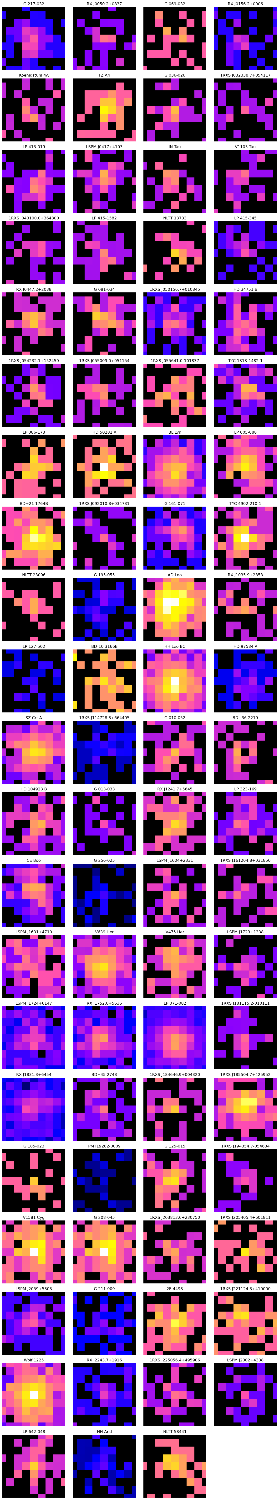
An important part of working with large datasets, be they of one object or multiple (as in this case) is memory management.
It might be tempting to load every image/exposure map into memory (and keep them there) as even laptops tend to have 8–16 GB of RAM at this point. Also, reading data from disk is slower than accessing it from memory.
However, memory saturation can creep up on you (with unpredictable consequences).
It’s important to get into good habits, even with an older mission like ROSAT whose data files are generally fairly small, and even with the relatively diminutive sample of M dwarfs we’re dealing with here.
As we’ve finished using the data associated with the pregenerated count-rate maps we can free up some RAM by deleting the data arrays.
We do make use of the exposure maps
to correct spectrum exposure times
later on in the demonstration, but because we’re using XGA product classes, the
exposure map data will be automatically re-loaded from disk when needed:
for cur_rt in pregen_ratemaps.values():
    # An upcoming XGA release includes better memory management, which
    #  will remove the necessity of much of this
    del cur_rt.image.data
    del cur_rt.expmap.data

    del cur_rt._data
    cur_rt._data = None
3. Generating new RASS images#
We’ve already made use of the pregenerated images included in the ROSAT All-Sky Survey archive, but what if we wanted to generate new versions? This section will take you through that process.
There are some practical limitations to what you can expect from RASS data:
Both the spatial and energy resolutions of ROSAT All-Sky Survey data are quite coarse; so if you want more finely binned images to tease out some spatial features, for instance, then be cautious.
Similarly, if you’re defining custom energy ranges, you will have to carefully consider the energy bounds you’re using so as to include enough spectral channels for there to be a usable number of photons in each pixel.
Making event lists easily accessible#
In preparation for the generation of our new RASS images (and the
extraction of new spectra
later on in this demonstration), we will load our skyfield event lists into XGA
EventList objects.
These objects won’t read the event list tables into memory, at least not automatically (we won’t be interacting with them through Python in this demonstration, so that data won’t be required).
Instead, they will provide a convenient interface to the event list headers:
preproc_event_lists = {}

for cur_src_name, cur_seq_id in src_seq_ids.items():
    cur_evt_path = PREPROC_EVT_PATH_TEMP.format(loi=cur_seq_id.lower())
    cur_evts = EventList(cur_evt_path, obs_id=cur_seq_id)
    cur_evts.src_name = cur_src_name

    preproc_event_lists[cur_src_name] = cur_evts

preproc_event_lists
{'CARMENES-2': <xga.products.misc.EventList at 0x7e4b3d8c23c0>,
 'CARMENES-35': <xga.products.misc.EventList at 0x7e4b3da88b60>,
 'CARMENES-37': <xga.products.misc.EventList at 0x7e4b3d1cee70>,
 'CARMENES-63': <xga.products.misc.EventList at 0x7e4b454cb4a0>,
 'CARMENES-64': <xga.products.misc.EventList at 0x7e4b3dfe5ca0>,
 'CARMENES-67': <xga.products.misc.EventList at 0x7e4b3db8d790>,
 'CARMENES-79': <xga.products.misc.EventList at 0x7e4b45427b90>,
 'CARMENES-103': <xga.products.misc.EventList at 0x7e4b3f1b5ee0>,
 'CARMENES-118': <xga.products.misc.EventList at 0x7e4b3db34c20>,
 'CARMENES-139': <xga.products.misc.EventList at 0x7e4b3f07e060>,
 'CARMENES-151': <xga.products.misc.EventList at 0x7e4b3d3ef560>,
 'CARMENES-155': <xga.products.misc.EventList at 0x7e4b3f233ad0>,
 'CARMENES-157': <xga.products.misc.EventList at 0x7e4b3f0b2870>,
 'CARMENES-161': <xga.products.misc.EventList at 0x7e4b44091010>,
 'CARMENES-168': <xga.products.misc.EventList at 0x7e4b3dd35250>,
 'CARMENES-169': <xga.products.misc.EventList at 0x7e4b3d15efc0>,
 'CARMENES-173': <xga.products.misc.EventList at 0x7e4b3d15fd10>,
 'CARMENES-174': <xga.products.misc.EventList at 0x7e4b3d2dfcb0>,
 'CARMENES-183': <xga.products.misc.EventList at 0x7e4b3de5b950>,
 'CARMENES-196': <xga.products.misc.EventList at 0x7e4b44093260>,
 'CARMENES-216': <xga.products.misc.EventList at 0x7e4b3d373590>,
 'CARMENES-224': <xga.products.misc.EventList at 0x7e4b3d1cdf40>,
 'CARMENES-226': <xga.products.misc.EventList at 0x7e4b44c2da00>,
 'CARMENES-233': <xga.products.misc.EventList at 0x7e4b44093e00>,
 'CARMENES-234': <xga.products.misc.EventList at 0x7e4b3d082330>,
 'CARMENES-266': <xga.products.misc.EventList at 0x7e4b3d094050>,
 'CARMENES-284': <xga.products.misc.EventList at 0x7e4b3d098140>,
 'CARMENES-301': <xga.products.misc.EventList at 0x7e4b3d0c39b0>,
 'CARMENES-307': <xga.products.misc.EventList at 0x7e4b3d0c0590>,
 'CARMENES-342': <xga.products.misc.EventList at 0x7e4b3cf10080>,
 'CARMENES-355': <xga.products.misc.EventList at 0x7e4b3d6ef350>,
 'CARMENES-358': <xga.products.misc.EventList at 0x7e4b440b7110>,
 'CARMENES-359': <xga.products.misc.EventList at 0x7e4b3d175880>,
 'CARMENES-363': <xga.products.misc.EventList at 0x7e4b3d674e00>,
 'CARMENES-371': <xga.products.misc.EventList at 0x7e4b3d675fd0>,
 'CARMENES-377': <xga.products.misc.EventList at 0x7e4b3d030740>,
 'CARMENES-378': <xga.products.misc.EventList at 0x7e4b3d54aa50>,
 'CARMENES-387': <xga.products.misc.EventList at 0x7e4b3d1a8da0>,
 'CARMENES-391': <xga.products.misc.EventList at 0x7e4b3d373cb0>,
 'CARMENES-396': <xga.products.misc.EventList at 0x7e4b3cf1df10>,
 'CARMENES-399': <xga.products.misc.EventList at 0x7e4b3d3d5130>,
 'CARMENES-411': <xga.products.misc.EventList at 0x7e4b3d061580>,
 'CARMENES-412': <xga.products.misc.EventList at 0x7e4b3cf35af0>,
 'CARMENES-413': <xga.products.misc.EventList at 0x7e4b44082000>,
 'CARMENES-417': <xga.products.misc.EventList at 0x7e4b3d0601a0>,
 'CARMENES-424': <xga.products.misc.EventList at 0x7e4b44083380>,
 'CARMENES-430': <xga.products.misc.EventList at 0x7e4b3d063a40>,
 'CARMENES-456': <xga.products.misc.EventList at 0x7e4b3d09a720>,
 'CARMENES-491': <xga.products.misc.EventList at 0x7e4b3d0c0470>,
 'CARMENES-517': <xga.products.misc.EventList at 0x7e4b3cf5d040>,
 'CARMENES-524': <xga.products.misc.EventList at 0x7e4b3d094080>,
 'CARMENES-526': <xga.products.misc.EventList at 0x7e4b3cf4fa40>,
 'CARMENES-537': <xga.products.misc.EventList at 0x7e4b3cf08da0>,
 'CARMENES-559': <xga.products.misc.EventList at 0x7e4b3d3b6060>,
 'CARMENES-561': <xga.products.misc.EventList at 0x7e4b3cf27bf0>,
 'CARMENES-563': <xga.products.misc.EventList at 0x7e4b3d3ed400>,
 'CARMENES-564': <xga.products.misc.EventList at 0x7e4b3cf726c0>,
 'CARMENES-578': <xga.products.misc.EventList at 0x7e4b3d39f1a0>,
 'CARMENES-585': <xga.products.misc.EventList at 0x7e4b440b7b60>,
 'CARMENES-594': <xga.products.misc.EventList at 0x7e4b44076600>,
 'CARMENES-603': <xga.products.misc.EventList at 0x7e4b3d059940>,
 'CARMENES-605': <xga.products.misc.EventList at 0x7e4b3d373680>,
 'CARMENES-613': <xga.products.misc.EventList at 0x7e4b3cf1e6c0>,
 'CARMENES-618': <xga.products.misc.EventList at 0x7e4b3cf8a8d0>,
 'CARMENES-630': <xga.products.misc.EventList at 0x7e4b3d033920>,
 'CARMENES-632': <xga.products.misc.EventList at 0x7e4b3cfafe60>,
 'CARMENES-633': <xga.products.misc.EventList at 0x7e4b44082570>,
 'CARMENES-641': <xga.products.misc.EventList at 0x7e4b3cf37230>,
 'CARMENES-645': <xga.products.misc.EventList at 0x7e4b440932c0>,
 'CARMENES-646': <xga.products.misc.EventList at 0x7e4b3cf379b0>,
 'CARMENES-669': <xga.products.misc.EventList at 0x7e4b440908c0>,
 'CARMENES-675': <xga.products.misc.EventList at 0x7e4b3cf4fc50>,
 'CARMENES-678': <xga.products.misc.EventList at 0x7e4b3cf0a510>,
 'CARMENES-681': <xga.products.misc.EventList at 0x7e4b3cfc0f80>,
 'CARMENES-694': <xga.products.misc.EventList at 0x7e4b3d0824e0>,
 'CARMENES-705': <xga.products.misc.EventList at 0x7e4b3cf5f290>,
 'CARMENES-708': <xga.products.misc.EventList at 0x7e4b3cf5fbf0>,
 'CARMENES-715': <xga.products.misc.EventList at 0x7e4b3d0c0d70>,
 'CARMENES-718': <xga.products.misc.EventList at 0x7e4b3d0c0140>,
 'CARMENES-724': <xga.products.misc.EventList at 0x7e4b3cf9a750>,
 'CARMENES-733': <xga.products.misc.EventList at 0x7e4b3d39d7c0>,
 'CARMENES-744': <xga.products.misc.EventList at 0x7e4b3cf73710>,
 'CARMENES-749': <xga.products.misc.EventList at 0x7e4b3d39f170>}
Defining energy bands for new images#
To make images with custom energy bounds, we need to know the mapping between the ROSAT-PSPC PI channels and energies, as the image generation tool we’re about to use wants us to specify channel bounds, rather than energy bounds.
The energy-channel scaling for ROSAT-PSPC is well known, and we have defined a
PSPC_EV_PER_CHAN Astropy Quantity constant in the Global Setup: Constants
section. You could also derive this value from the ROSAT-PSPCC Redistribution
Matrix File (RMF), which describes the relationship between
channels and energy - we fetch the RMF in a later section.
Now we get to define the energy bounds for the images we want to generate.
As we’ve previously mentioned, RASS’ energy range is quite limited by modern standards, only 0.07–2.4 keV. For this demonstration we make new images in two energy bands; 0.5–2.0 keV and 1.0–2.0 keV.
The 0.5–2.0 keV band is often referred to as the ‘soft band’, at least in X-ray galaxy cluster studies (every field seems to have its own definition of what ‘soft’ means), and might be useful for comparisons to images from other missions.
rass_im_en_bounds = Quantity([[0.5, 2.0], [1.0, 2.0]], "keV")
Note
If you run this demonstration with a modified rass_im_en_bounds variable, note that
even a single energy band should be defined as though it were part of a list
(e.g., Quantity([[0.5, 2.0]], "keV")), to make it compatible with the image
generation function we use later in the notebook.
Converting those energy bounds to channel bounds is straightforward, we simply divide the energy values by our assumed mapping between energy and channel.
The resulting lower and upper bound channel values are rounded down and up to the nearest integer channel respectively.
rass_im_ch_bounds = (rass_im_en_bounds / PSPC_EV_PER_CHAN).to("chan")
rass_im_ch_bounds[:, 0] = np.floor(rass_im_ch_bounds[:, 0])
rass_im_ch_bounds[:, 1] = np.ceil(rass_im_ch_bounds[:, 1])
rass_im_ch_bounds = rass_im_ch_bounds.astype(int)
rass_im_ch_bounds
Note
Though we demonstrate how to convert energy bounds to channel bounds above, the wrapper function for image generation will repeat this exercise, as it will write energy bounds into output file names.
Image binning factor#
The final choice we have to make before generating new images is the ‘binning factor’ (or factors). These control the spatial resolution of the output images, and are essentially the number of RASS’ Sky X-Y ‘pixels’ that get binned into a single output image pixel.
Archived RASS images were created with a binning factor of 90, resulting in a 512x512 grid, and a pixel scale of 45\(^{\prime\prime}\).
Calculating the binning factor required for a particular image pixel scale is quite straightforward. We can pull the intrinsic Sky X-Y pixel scale from the header of an events list, then divide our desired pixel scale by that number.
As we’re extracting the Sky X-Y pixel scale from only the TCDLT1 entry (there is another equivalent value for the y-direction stored under TCDLT2) there is an implicit assumption here that the Sky X-Y pixels are square, but that is reasonable.
Here we demonstrate calculating the binning factor for a pixel scale of
\(1^{\prime}\); the chain of method calls (.to('').round(0).astype(int).value)
applied to the calculation:
Ensures the Astropy quantity result is dimensionless, rather than in units of \(\frac{\prime}{\circ}\).
Rounds to the nearest integer.
Converts the data type to integer and then reads out the integer value from the Astropy quantity.
cur_evts = list(preproc_event_lists.values())[0]
cur_skyxy_ps = abs(Quantity(cur_evts.event_header["TCDLT1"], "deg/pix"))

calc_ibf = (Quantity(1, "arcmin/pix") / cur_skyxy_ps).to("").round(0).astype(int).value
calc_ibf
np.int64(120)
We have somewhat arbitrarily chosen two coarser binning factors for this demonstration, corresponding to pixel scales of \(90^{\prime\prime}\) and \(135^{\prime\prime}\) respectively:
# List of binning factors for the new images
bin_factors = [180, 270]
Danger
Choosing very small values for the binning factor, for instance 1, will mean that generation of new images will consume a great deal of memory, and output files will be very large.
Incidentally, there would be very little point to generating images at the Sky X-Y pixel scale for RASS, as it would dramatically oversample the practical angular resolution of the survey.
Running image generation#
There is no HEASoft tool specifically intended to generate RASS images, but there is a generalized HEASoft image (and other data product) generation task that we can use.
If you have previously generated images, light curves, or spectra from HEASARC-hosted
X-ray data on the command line, you may well have come across XSELECT; a HEASoft
tool for interactively generating data products from event lists.
When creating data products, XSELECT calls the HEASoft extractor task, which we
will now use to demonstrate the creation of RASS images.
As with all uses of HEASoft tasks in this notebook, our call to extractor will be
through the HEASoftPy Python interface - specifically the hsp.extractor function.
We have implemented a wrapper to this function in the Global Setup: Functions section of this notebook, primarily so that we can easily run the generation of new images in parallel:
arg_combs = [
    [
        cur_evts.path,
        os.path.join(SEQ_OUT_PATH, cur_evts.obs_id),
        cur_evts.obs_id,
        *cur_bnds,
        cur_bf,
    ]
    for cur_evts in preproc_event_lists.values()
    for cur_bnds in rass_im_en_bounds
    for cur_bf in bin_factors
]

with mp.Pool(NUM_CORES) as p:
    im_result = p.starmap(gen_rass_image, arg_combs)
/opt/envs/heasoft/lib/python3.12/multiprocessing/popen_fork.py:66: DeprecationWarning: This process (pid=875) is multi-threaded, use of fork() may lead to deadlocks in the child.
  self.pid = os.fork()
Example visualization of new images#
To show off the various images we just created for each RASS skytile relevant to our M dwarf sample, we create a figure that displays them in a grid; each column corresponds to a different energy band, and each row to a different binning factor:
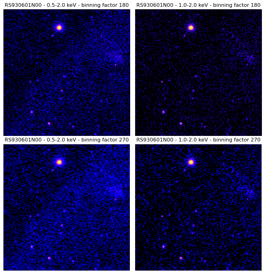
4. Generating RASS spectra for our sample#
The image data products we generated in the previous section were general, valid for any source that happens to be within those skytiles. It might not even be necessary to make new skytile images for your science case, the archived images could well be sufficient.
Now, though, we generate spectra - these data products are specific to the sources we want to study and are not contained in the RASS archive.
The energy resolution/range of ROSAT All-Sky Survey data is quite limited, as was the sensitivity of the PSPC instrument and the average exposure time across the survey.
However, as we’ve previously stated, this is still the only publicly available imaging X-ray dataset across the entire sky - it is quite possible that RASS spectra can still lend insight to your research.
Defining the size of source and background regions#
To make a useful spectrum, we have to define a spatial region that we have decided will contain photons emitted by our source. That will have to be done for each source we want to study.
For this particular demonstration, we will also define another region per M dwarf, which
will define where the background spectrum is extracted from. Though there are other methods
for handling the ROSAT-PSPC background
(the pcparpha
tool will generate particle background spectra for ROSAT-PSPC, for instance), they are
outside the scope of this demonstration.
In a more complex case - for instance, if we were studying an extended source like a galaxy cluster or a supernova remnant - we might also have to worry about excluding regions unrelated, contaminating, sources. That is outside the scope of this getting started guide, however, and we do not exclude any regions in this demonstration.
This tutorial creates identically sized source and background regions for each source
in our sample. Source regions are circles, with their angular radii set to the value of
SRC_ANG_RAD, centered on the CARMENES RA-Dec coordinate; background regions are also
centered on the CARMENES coordinate, but are circular annuli, with inner radii set to
INN_BACK_FACTOR\(\times\)SRC_ANG_RAD and outer radii set
to OUT_BACK_FACTOR\(\times\)SRC_ANG_RAD:
SRC_ANG_RAD = Quantity(2, "arcmin")

INN_BACK_FACTOR = 1.05
OUT_BACK_FACTOR = 1.5
You could alter the values above to adjust the size of the regions for your own use. It would also be straightforward to modify the setting up Astropy regions section to be able to specify different region sizes for different sources.
Constructing RA-Dec ↔ RASS sky pixel WCSes#
In the previous section, we talked about defining the size and location of source/background regions in terms of angular radius and RA-Dec central coordinates.
Unfortunately, the extractor tool we’re going to use to make our spectra wants us to
pass regions that are in the RASS Sky X-Y coordinate system (there can be issues
with the generation of ‘weighting maps’ for RASS data if not) - so we need to make
sure that we’re able to convert from RA-Dec to Sky X-Y.
Luckily for us, the RASS event lists we’ll be creating new spectra from contain the necessary information to construct Astropy World Coordinate System (WCS) objects that can do just that.
Here we set up one WCS per skytile (which is the same thing as saying one per source
in this case) and store them in a dictionary for later access and use. The following
information is being pulled from the event list’s STDEVT table header (through
an XGA EventList object):
Pixel scale - One entry per direction (i.e., X and Y), and assigned to the
cdeltproperty, these describe how many degrees a single RASS Sky X-Y pixel step corresponds to.Critical pixel - An X-Y pixel coordinate that acts as a reference point for how Sky X-Y coordinates map onto RA-Dec coordinates, works in concert with the next entry.
RA-Dec at critical pixel - The RA-Dec coordinate corresponding to the Sky X-Y coordinate defined by the previous entry.
Sky X-Y ↔ RA-Dec projection - Which projection is used to map the cartesian Sky X-Y coordinate system onto the spherical RA-Dec coordinate system.
radec_skyxy_wcses = {}

for cur_src_name, cur_evts in preproc_event_lists.items():
    cur_wcs = WCS(naxis=2)
    cur_wcs.wcs.cdelt = [
        cur_evts.event_header["TCDLT1"],
        cur_evts.event_header["TCDLT2"],
    ]

    cur_wcs.wcs.crpix = [
        cur_evts.event_header["TCRPX1"],
        cur_evts.event_header["TCRPX2"],
    ]

    cur_wcs.wcs.crval = [
        cur_evts.event_header["TCRVL1"],
        cur_evts.event_header["TCRVL2"],
    ]

    cur_wcs.wcs.ctype = [
        cur_evts.event_header["TCTYP1"],
        cur_evts.event_header["TCTYP2"],
    ]

    radec_skyxy_wcses[cur_src_name] = cur_wcs
Setting up Astropy regions representing source and background regions#
We are now ready to set up our source and background regions; first in RA-Dec coordinates (with angular radii), and then also in Sky X-Y coordinates (and sky pixel radii).
The latter regions will be saved to disk as region files and ultimately passed to the
HEASoft extractor tool when we create our new spectra.
In order to simplify the definition of these regions, we will use the
Astropy-affiliated regions module. It’s also
worth considering that this approach scales well to more complicated cases where
we need to exclude a set of contaminating regions before we extract a spectrum.
Iterating through each source in our sample, we:
Fetch the appropriate WCS for the current source (set up in the previous section).
Fetch the CARMENES RA-Dec coordinate for the current source.
Create an Astropy
CircleSkyRegioninstance, centered on the CARMENES RA-Dec, with a radius taken fromSRC_ANG_RAD, and store it in a dictionary for later.Repeat the last step but instantiate a
CircleAnnulusSkyRegionfor the background region, with an inner radius ofINN_BACK_FACTOR\(\times\)SRC_ANG_RADand an outer radius ofOUT_BACK_FACTOR\(\times\)SRC_ANG_RAD.Convert both source and background regions to the Sky X-Y coordinate system and write them to disk as DS9-formatted region files.
src_bck_radec_regs = {n: {"src": None, "bck": None} for n in src_seq_ids.keys()}
src_bck_skyxy_reg_files = {n: {"src": None, "bck": None} for n in src_seq_ids.keys()}

for cur_src_ind, cur_name_wcs in enumerate(radec_skyxy_wcses.items()):
    cur_src_name, cur_wcs = cur_name_wcs

    cur_src_coord = matched_carm_coords[cur_src_ind]

    cur_src_radec_reg = CircleSkyRegion(cur_src_coord, SRC_ANG_RAD)
    src_bck_radec_regs[cur_src_name]["src"] = cur_src_radec_reg

    cur_bck_radec_reg = CircleAnnulusSkyRegion(
        cur_src_coord, SRC_ANG_RAD * INN_BACK_FACTOR, SRC_ANG_RAD * OUT_BACK_FACTOR
    )
    src_bck_radec_regs[cur_src_name]["bck"] = cur_bck_radec_reg

    # Convert to Sky X-Y coordinates
    cur_src_skyxy_reg = cur_src_radec_reg.to_pixel(cur_wcs)
    cur_bck_skyxy_reg = cur_bck_radec_reg.to_pixel(cur_wcs)

    # Write Sky X-Y regions to files
    os.makedirs(os.path.join(SRC_OUT_PATH, cur_src_name), exist_ok=True)

    cur_src_skyxy_reg_path = SRC_REG_PATH_TEMP.format(
        sn=cur_src_name, oi=src_seq_ids[cur_src_name]
    )
    with open(cur_src_skyxy_reg_path, "w") as srco:
        srco.write(
            Regions([cur_src_skyxy_reg])
            .serialize(format="ds9")
            .replace("image", "physical")
        )
    src_bck_skyxy_reg_files[cur_src_name]["src"] = cur_src_skyxy_reg_path

    cur_bck_skyxy_reg_path = BCK_REG_PATH_TEMP.format(
        sn=cur_src_name, oi=src_seq_ids[cur_src_name]
    )
    with open(cur_bck_skyxy_reg_path, "w") as bcko:
        bcko.write(
            Regions([cur_bck_skyxy_reg])
            .serialize(format="ds9")
            .replace("image", "physical")
        )
    src_bck_skyxy_reg_files[cur_src_name]["bck"] = cur_bck_skyxy_reg_path
Note
During the preparation of the RASS Sky X-Y coordinate system region files using the
Astropy-affiliated regions module, we generate a serialization (the string contents
of the final file) of each region, rather than simply writing directly to disk using
`Regions([…]).write(region file path, format).
This is because we need to replace the coordinate system name that is automatically
used for all non-RA-Dec files written by the regions module (image), with
physical, which is what the extractor tool will be expecting.
Defining image binning for the ‘weighting maps’#
As it turns out, when we create a new spectrum with HEASoft’s extractor task, we’re
also generating an image and storing it in a FITS image extension of the
spectrum file.
The new image stored in each spectrum is a ‘weighted map’ (or ‘WMAP’, and no not the CMB observatory), and will be used during the generation of Ancillary Response Files (ARFs).
ARFs describe the ‘effective area’ (i.e., sensitivity) as a function of incident-photon-energy. The ARFs used during normal analyses are a combination of the X-ray optics’ (called the X-ray Mirror Assembly, or XMA, for ROSAT) and the energy-dependent efficiency of the detector.
A WMAP is essentially the same as a ‘normal’ X-ray image and allows ARF calculation to find the average of ROSAT-PSPC response across the source region, weighted by the number of photons arriving at each point.
Weighted ARF calculation is particularly important for scanning-mode observations such as those that comprise the ROSAT All-Sky Survey, as the X-ray sky is drifting through the PSPCC FoV, see Belloni T., et al. (1994) for a discussion. Using the WMAP in ARF generation is meant to help account for this movement across the instrument, but its efficacy has not been well explored.
Also worth noting is that weighting ARFs is also very important for the analysis of extended sources (true of all spectro-imaging X-ray missions), though we are treating all our M dwarfs as point sources for this tutorial.
All that said, we need to choose a binning factor (the same idea as when we generated new images in the last section) for the WMAPs that will be generated with our new spectra. We select the same binning factor as was used to make archived RASS images; you may wish to experiment with different values to see how they affect the resulting ARFs.
wmap_bin_factor = 90
Running spectrum generation#
Here we run the actual generation of spectra for each M dwarf in our sample; just like with our image generation, individual products will be generated in parallel, maximizing the use of our computing resources and saving us some time.
The creation of new spectra from ROSAT All-Sky Survey data is achieved through the
use of HEASoft’s extractor task (again, just like our image generation) - this
demonstration uses the Python interface provided by HEASoftPy; hsp.extractor(...).
We have set up a wrapper function, gen_rass_spectrum(...), to generate RASS spectra
in the ‘Global Setup: Functions’ section of this notebook, mostly to make
it easier to parallelize.
Now we generate one source, and one background, spectrum per M dwarf, passing paths to the region files we set up, the RA-Dec source region object (so that coordinates and radius can be extracted and included in the file name), and the binning factor we defined above:
arg_combs = [
    [
        cur_evts.path,
        os.path.join(SRC_OUT_PATH, cur_name),
        cur_evts.obs_id,
        cur_name,
        src_bck_radec_regs[cur_name]["src"],
        src_bck_skyxy_reg_files[cur_name]["src"],
        src_bck_skyxy_reg_files[cur_name]["bck"],
        wmap_bin_factor,
    ]
    for cur_name, cur_evts in preproc_event_lists.items()
]

with mp.Pool(NUM_CORES) as p:
    sp_result = p.starmap(gen_rass_spectrum, arg_combs)
/opt/envs/heasoft/lib/python3.12/multiprocessing/popen_fork.py:66: DeprecationWarning: This process (pid=875) is multi-threaded, use of fork() may lead to deadlocks in the child.
  self.pid = os.fork()
Important
Technically the ROSAT-PSPC PI channel range goes up to 500, but only the
first 256 are actually usable for analysis. Still, extractor(...) would
create 500-channel spectra if you let it, and those files would be incompatible
with 256-channel RMF we will fetch in the next section.
As such, the file path passed to extractor in the gen_rass_spectrum() function
(see the ‘Global Setup: Functions’ section of this notebook), has a
channel filter command appended to it - “[PI=0:256]”. This ensures that only the
valid channels are considered, and makes the spectrum compatible with the RMF.
Generating supporting files#
A spectrum tells us how many photons were observed by ROSAT-PSPC in each detector channel, but to turn that into information about what was emitted by a source, we need a couple more data products.
Redistribution Matrix File (RMF)#
RMFs describe how a detector’s channels correspond to the energies of incident photons - knowing that takes the spectrum from photons observed in a particular channel, to photons observed at a particular energy.
That is clearly useful, as different astrophysical processes can be responsible for different photon energies, and we need an energy spectrum in our observer’s frame to be able to explore the source’s rest frame spectrum.
For RASS, we need to fetch the ROSAT-PSPCC RMF from the
HEASARC Calibration Database (CALDB). HEASoft’s quzcif
tool (we’re using the HEASoftpy interface) allows us to query the HEASARC CALDB for
specific files - it can both return the names of matching files and download the file
itself.
Many arguments can be passed to this tool to narrow down the files that are returned, including the name of the mission, instrument, and the type of CALDB file we’re looking for.
In this case we set mission="rosat" (of course), the instrument as ‘pspcc’ (as
ROSAT-PSPCC was used for the all-sky survey, and PSPCB for pointed
observations), and the CALDB codename="MATRIX" (RMFs are stored under this codename).
The only other argument we pass to filter the search results is expr="pich.eq.256"; this
translates as “return matching files where a PI channel boundary is equal to 256”. In this
case 256 is the upper boundary of the valid PI range of the RMF we wish to retrieve.
ROSAT’s CALDB entry includes a PROS 34-channel variant of the RMF, which would be invalid for our purposes. It is important to know, though, that the 256-channel RMF greatly oversamples the energy response of the PSPC. The 34-channel PROS response is a better match to the intrinsic energy resolution.
As we set retrieve=True the RMF will be downloaded to our current directory, so we
use a context manager that temporarily changes the working directory to
ROOT_DATA_DIR, and set up a variable containing the path to the freshly acquired RMF:
# This will find and download (retrieve=True) the ROSAT-PSPCC RMF file for
#  the 256 standard channel data
with contextlib.chdir(ROOT_DATA_DIR):
    caldb_rmf_ret = hsp.quzcif(
        mission="rosat",
        instrument="pspcc",
        codename="MATRIX",
        filter="-",
        date="-",
        time="-",
        expr="pich.eq.256",
        noprompt=True,
        retrieve=True,
        clobber=True,
    )

    # Store the path to the downloaded RMF in a variable, we'll use this later
    single_rmf_path = os.path.join(ROOT_DATA_DIR, caldb_rmf_ret.output[0].split(" ")[0])
Important
RMFs fundamentally describe the calibration of an instrument’s channels and event
energies. Both the understanding of that calibration, and the behaviors of the
instrument itself, often evolve with time. As such, if you are retrieving other RMFs
using quzcif you should set the time and date filters to ensure you retrieve a file
that matches your observation.
We do not set times and dates here because only one RMF was released for ROSAT-PSPCC, as the instrument was destroyed fairly early in the mission’s lifetime.
We just downloaded the appropriate RMF for RASS, so now we’ll make a copy for each spectrum we’ve generated (a little wasteful, but it is a small file):
rmf_paths = []

for cur_src_name, cur_seq_id in src_seq_ids.items():
    out_rmf_path = RMF_PATH_TEMP.format(oi=cur_seq_id, sn=cur_src_name)
    copyfile(single_rmf_path, out_rmf_path)

    rmf_paths.append(out_rmf_path)
Ancillary Response Files (ARF)#
HEASoft’s pcarf task is specifically intended to make ARFs for ROSAT-PSPC data, so
we will make good use of it!
We discussed what ARFs are in an earlier section - the benefit of understanding the instrument’s sensitivity as a function of energy is that we can model what the original ‘real’ spectrum emitted by the source would have to be, to match the spectrum said instrument has observed.
That modeling is basically what X-ray spectral fitting is all about - various tools exist to perform the task, but in Section 5 we’ll use the PyXSPEC module.
We wish to parallelize the generation of ARFs for different spectra, and so create a
wrapper function (gen_rosat_pspc_arf(...), see the ‘Global Setup: Functions’ section)
around the pcarf task to make that easier.
The inputs are very limited, only the directory to write the ARF to, the path to the
source spectrum file (extracted from the return of the spectrum generation
step; sp_result[cur_ind][2]), and a path to the RMF file are required (the RMF path
can also be set to ‘CALDB’ to automatically acquire it for this process):
arg_combs = [
    [
        os.path.join(SRC_OUT_PATH, cur_name),
        sp_result[cur_ind][2],
        single_rmf_path,
    ]
    for cur_ind, cur_name in enumerate(preproc_event_lists)
]

with mp.Pool(NUM_CORES) as p:
    arf_result = p.starmap(gen_rosat_pspc_arf, arg_combs)
Correcting RASS exposure times in spectral files#
An important quirk of ROSAT All-Sky Survey data is that the ‘LIVETIME’ information (the amount of time the detector was ‘on source’ and collecting data) contained in the event list is unhelpful/incorrect in two ways:
It reports the total ‘live time’ for the entire skytile, which was observed in many passes; this means a much larger live time than was actually spent on a source.
The live time entry is deliberately negative (e.g., a whole-skytile livetime of 17961 s is reported as -17961 s) to ensure it isn’t accidentally used in analyses.
Our newly generated spectra will have inherited that incorrect information, and so we need to fix it.
Thankfully, that’s pretty straightforward; we can use the exposure maps included in the archived RASS data directories (the contents of which we discussed in a previous section) to look up the actual exposure time at the coordinates of each spectrum’s source.
Exposure times at source coordinates are fetched from the ExpMap instances we
set up earlier by passing the relevant
source coordinate to the get_exp(...) method.
The FITS headers of the source and background spectra are then updated so that the “EXPOSURE” entry is set to the newly extracted exposure time:
for cur_ind, cur_src_name in enumerate(preproc_event_lists):

    cur_sp_path = sp_result[cur_ind][2]
    cur_bsp_path = sp_result[cur_ind][3]

    cur_coord = matched_carm_coords[cur_ind]
    cur_coord_quan = Quantity([cur_coord.ra, cur_coord.dec], "deg")

    cur_ex = pregen_ratemaps[cur_src_name].expmap
    del cur_ex.data
    cur_exp_time = cur_ex.get_exp(cur_coord_quan)

    with fits.open(cur_sp_path, mode="update") as speco:
        for en in speco:
            if "EXPOSURE" in en.header:
                del en.header["EXPOSURE"]
            en.header["EXPOSURE"] = cur_exp_time.to("s").value.round(5)

    with fits.open(cur_bsp_path, mode="update") as bspeco:
        for en in bspeco:
            if "EXPOSURE" in en.header:
                del en.header["EXPOSURE"]
            en.header["EXPOSURE"] = cur_exp_time.to("s").value.round(5)
Grouping spectral channels#
RASS spectra are likely to be low signal-to-noise due to the small effective area of ROSAT-PSPC (relative to many modern missions), and the short mean exposure time of the survey (~400 s). That said, due to the scanning pattern of the ROSAT All-Sky Survey, the ecliptic pole regions have considerably longer total exposure times. As such, sources in these regions (the Magellanic Clouds, for instance) can have quite high signal-to-noise compared to the rest of the sky.
As such, it is normally going to be a good idea to ‘group’ the channels of a RASS spectrum; combining sequential channels into a single bin until a particular quality metric is reached (e.g., a minimum number of counts, or a minimum signal-to-noise).
Some missions have created their own tools to perform this task, but HEASoft includes
a generalized task called ftgrouppha that can be applied to any spectrum.
Several grouping metrics are implemented in ftgrouppha; we’ll take the simplest
option and require a minimum number of counts per channel. The following will
be passed to the task and will group channels until there are at least three counts:
spec_group_type = "min"
spec_group_scale = 3
Now we will apply ftgrouppha to each source spectrum, and save the output as a new
grouped spectrum file. That grouped spectrum file is what will be used for model
fitting in Section 5.
Grouping a spectrum in this manner is not particularly computationally expensive, so
we have not bothered to write a wrapper function for ftgrouppha and parallelize the
process as we did for the product generation tasks. Note, however, that if you are
working on a much larger sample, you may want to take the time to parallelize this step.
The paths to the initial spectra are retrieved from the output of the spectrum
generation step (sp_result[cur_ind][2]), and the paths to the output files are
stored in a dictionary (grouped_sp_paths) for later use:
grp_spec_paths = {}

for cur_ind, cur_src_name in enumerate(preproc_event_lists):

    cur_sp_path = sp_result[cur_ind][2]

    cur_grp_spec = cur_sp_path.replace(
        "-spectrum", f"-{spec_group_type}grp{spec_group_scale}-spectrum"
    )

    hsp.ftgrouppha(
        infile=cur_sp_path,
        outfile=cur_grp_spec,
        grouptype=spec_group_type,
        groupscale=spec_group_scale,
        clobber=True,
        chatter=TASK_CHATTER,
        noprompt=True,
    )

    grp_spec_paths[cur_src_name] = cur_grp_spec
Adding supporting file paths to spectrum headers#
The very last thing we want to do before we can fit models to our spectra is to alter their FITS headers so they point to the ARF, RMF, and background files.
We don’t absolutely need to do this, as the paths to supporting files can be manually passed to PyXSPEC (and command-line XSPEC) as the data are loaded in.
However, including the paths in the headers means the ARF, RMF, and background spectra can be loaded in automatically, so we might as well:
for cur_ind, cur_src_name in enumerate(preproc_event_lists):

    cur_gsp_path = grp_spec_paths[cur_src_name]
    cur_bsp_path = sp_result[cur_ind][3]

    cur_arf_path = arf_result[cur_ind][1]
    cur_rmf_path = rmf_paths[cur_ind]

    with fits.open(cur_gsp_path, mode="update") as speco:

        del speco["SPECTRUM"].header["RESPFILE"]
        speco["SPECTRUM"].header["RESPFILE"] = os.path.basename(cur_rmf_path)

        del speco["SPECTRUM"].header["ANCRFILE"]
        speco["SPECTRUM"].header["ANCRFILE"] = os.path.basename(cur_arf_path)

        del speco["SPECTRUM"].header["BACKFILE"]
        speco["SPECTRUM"].header["BACKFILE"] = os.path.basename(cur_bsp_path)
Caution
We add the RESPFILE, ANCRFILE, and BACKFILE keywords after grouping because some
FITS file modifications (such as using ftgrouppha) can add ‘&’ characters to the end
of long strings in FITS headers. That then causes PyXSPEC to fail to read in supporting
files for the spectrum.
As HEASARC-tutorials demonstrations lean toward using easy-to-read, informative, file names that are by necessity quite long, we add the correct paths using the Astropy fits module.
5. Fitting spectral models using PyXSPEC#
Having gone to the trouble of generating ROSAT All-Sky Survey spectra for our sample of M dwarfs, we’ll now fit some models and try to extract some properties!
Using the Python interface (PyXSPEC) to the ubiquitous XSPEC model fitting software, we will:
Fit both power-law and blackbody models to each spectrum.
Calculate and store the model fluxes.
Extract and store the model parameters and uncertainties.
Prepare to create visualizations of the fitted spectra.
Note that this demonstration was not written by an expert in the X-ray emission of M dwarfs (or indeed any kind of star), so please don’t necessarily take these models as a recommendation for your own work!
Setting up PyXSPEC#
Firstly, we configure how PyXSPEC is going to behave. This includes:
Setting the ‘chatter’ to zero, to minimize the outputs that XSPEC prints. Note that, at the time of writing, there are some PyXSPEC outputs that cannot be suppressed.
Telling PyXSPEC to use the Cash statistic; generally considered a good choice for low-count spectra.
Making sure that PyXSPEC won’t ask us for input at any point (
xs.Fit.query = "no").
# The strange comment on the end of this line is for the benefit of our
#  automated code-checking processes. You shouldn't import modules anywhere but
#  the top of your file, but this is unfortunately necessary at the moment
import xspec as xs  # noqa: E402

# Limits the amount of output from XSPEC that PyXspec will display
xs.Xset.chatter = 0

# Other xspec settings
xs.Plot.area = True
xs.Plot.xAxis = "keV"
xs.Plot.background = True
xs.Fit.statMethod = "cstat"
xs.Fit.query = "no"
xs.Fit.nIterations = 500
We also define a variable that will control whether warnings of our own creation are displayed; see the code cell in the next section. By default, we will not display those warnings, but the possible problems they describe will still be dealt with:
show_warn = False
Loading spectra and fitting models#
This section contains the entirety of our interaction with PyXSPEC in this notebook; the slightly ugly for loop below will load each spectrum individually, restrict the energy range, fit models, and create the visualization data (though it won’t plot it).
What we’re doing here represents a fairly simple use of PyXSPEC; some of our other demonstrations, such as ‘Getting started with Swift-XRT, contain more complex examples; the simultaneous fitting of a model to multiple spectra, for instance.
The most important steps are:
Once a spectrum is loaded, we restrict our analysis to data points between 0.11–2.02 keV, also excluding any marked as ‘bad’ by
ftgrouppha.Plotting information for the data is then generated and stored for later.
We move on to model fitting only if \(>2\) channels are valid (very low SNR spectra may have one or two); having the same number of channels (or fewer) as there are model parameters would mean an invalid fit.
Looping through models (power law and blackbody in this case), they are fit to the data (using default starting parameter values), parameter errors and then model fluxes are calculated, and the results are stored in dictionaries.
Plotting information for the models is generated and stored for later.
Finally, the dictionaries of model parameters, uncertainties, and fluxes for each source are combined into Pandas DataFrames, for easier visualization, interaction, and saving.
The low SNR of some of these spectra will almost inevitably lead to poor fits in some
cases, or cause trouble calculating model parameter uncertainties. We keep an eye out
for the latter case especially, as we can use a string returned by XSPEC’s error
command to check if it has flagged any potential problems with the uncertainties.
We can display a warning when this happens (the visibility of which is controlled
by the show_warn variable defined in the last section), but
we always write a boolean value to the storage dictionaries indicating if there were
problems with a particular model parameter’s uncertainty calculation.
spec_plot_data = {}
fit_plot_data = {}
fit_parameters = {}
fit_fluxes = {}

# Iterating through all the ObsIDs
with tqdm(desc="PyXspec - loading RASS spectra", total=len(grp_spec_paths)) as onwards:
    for gsp_ind, cur_name_spec in enumerate(grp_spec_paths.items()):
        cur_src_name, cur_grp_spec = cur_name_spec

        xs.AllData.clear()
        xs.AllModels.clear()

        with contextlib.chdir(os.path.dirname(cur_grp_spec)):
            xs.AllData(cur_grp_spec)
            spec = xs.AllData(1)

        spec.ignore("**-0.11 2.02-**")
        xs.AllData.ignore("bad")

        num_chan_noticed = len(xs.AllData(1).noticed)

        xs.Plot()
        spec_plot_data[cur_src_name] = [
            xs.Plot.x(1),
            xs.Plot.xErr(1),
            xs.Plot.y(1),
            xs.Plot.yErr(1),
        ]

        fit_parameters.setdefault(cur_src_name, {})
        fit_fluxes.setdefault(cur_src_name, {})
        if num_chan_noticed > 2:
            fit_plot_data.setdefault(cur_src_name, {})

            for cur_model_name in ["bbody", "powerlaw"]:

                xs.Model(cur_model_name)
                xs.Fit.perform()

                xs.Plot()
                fit_plot_data[cur_src_name][cur_model_name] = xs.Plot.model(1)

                xs.Fit.error("2.706 1 2")

                xs.AllModels.calcFlux("0.5 2.0 err")
                en_fl, en_fl_min, en_fl_max, ph_fl, ph_fl_min, ph_fl_max = spec.flux

                fit_fluxes[cur_src_name].update(
                    {
                        f"{cur_model_name}_0.5-2.0keV_flux": en_fl,
                        f"{cur_model_name}_0.5-2.0keV_flux_err-": en_fl_min,
                        f"{cur_model_name}_0.5-2.0keV_flux_err+": en_fl_max,
                    }
                )

                for cur_par_id in range(1, xs.AllModels(1).nParameters + 1):
                    cur_par_name = xs.AllModels(1)(cur_par_id).name

                    cur_par_val = xs.AllModels(1)(cur_par_id).values[0]
                    cur_par_lims_out = xs.AllModels(1)(cur_par_id).error

                    # Check the error string output by XSPEC's error command and
                    #  show a warning if there might be a problem
                    error_good = True
                    if cur_par_lims_out[2] != "FFFFFFFFF":
                        if show_warn:
                            warn(
                                f"Error calculation for the {cur_par_name} parameter "
                                f"of {cur_model_name} indicated a possible problem "
                                f"({cur_par_lims_out[2]}) [{cur_src_name}]",
                                stacklevel=2,
                            )
                        error_good = False

                    fit_parameters[cur_src_name].update(
                        {
                            f"{cur_model_name}_{cur_par_name}": cur_par_val,
                            f"{cur_model_name}_{cur_par_name}_err-": cur_par_val
                            - cur_par_lims_out[0],
                            f"{cur_model_name}_{cur_par_name}_err+": cur_par_lims_out[1]
                            - cur_par_val,
                            f"{cur_model_name}_{cur_par_name}_good_err": error_good,
                        }
                    )

        onwards.update(1)

fit_parameters = pd.DataFrame.from_dict(fit_parameters, orient="index")
fit_fluxes = pd.DataFrame.from_dict(fit_fluxes, orient="index")
Note
We ignore any channels that are outside the 0.11-2.02 keV energy range, which was
chosen using advice from the ROSAT-PSPC energy calibration table. Any channels
that have been marked as ‘bad’ by ftgrouppha are also excluded.
Visualizing fitted spectra#
At this stage we have fitted two models to most of the spectra (those with \(<3\) valid channels were excluded). We now might want to take a look at them plotted on top of the spectrum they were fitted to (we also have the necessary data to plot those spectra with no model fits).
We set up a many-panel figure to display the fitted, background-subtracted, spectrum for each of our M dwarfs. The x-axis energy scales are consistent across all panels, and the y-axis scale is consistent across rows.
Here we set up the colors assigned to each model:
nice_model_names = {"bbody": "Blackbody", "powerlaw": "Power-law"}
nice_model_colors = {"bbody": "firebrick", "powerlaw": "teal"}

Saving PyXSPEC fit results#
If you’re fitting X-ray spectra as part of a research project, you’re probably going to want to save the properties you derived to a file, so you can use them later without re-running the analysis.
In the section where we
loaded and fit the spectra, we mentioned
converting the parameter storage dictionaries into Pandas DataFrame objects, one for
fluxes (fit_fluxes) and another for model parameters and
uncertainties (fit_parameters).
Here we combine them into a single dataframe by performing a table merge, matching the dataframe indexes (which, due to the way we created the dataframes, are the “CARMENES-{ID}” style names we assigned to each source earlier).
fit_parameters = fit_parameters.round(5)
fit_fluxes = fit_fluxes.round(16)
rass_results = pd.merge(fit_parameters, fit_fluxes, left_index=True, right_index=True)

rass_results = pd.merge(
    carm_cat.to_pandas()[["Karmn", "Name", "id_name"]],
    rass_results,
    right_index=True,
    left_on="id_name",
)

rass_results = rass_results.set_index("id_name")
The combined dataframe is then saved as a comma-separated values (CSV) file:
# Using a convenience method of the Pandas DataFrame class
rass_results.to_csv("carmenes_mdwarf_rass_properties.csv", index=True)
We can also take a peek at the first few rows, to see what information it contains:
rass_results.head(6)
| Karmn | Name | bbody_kT | bbody_kT_err- | bbody_kT_err+ | bbody_kT_good_err | bbody_norm | bbody_norm_err- | bbody_norm_err+ | bbody_norm_good_err | ... | powerlaw_norm | powerlaw_norm_err- | powerlaw_norm_err+ | powerlaw_norm_good_err | bbody_0.5-2.0keV_flux | bbody_0.5-2.0keV_flux_err- | bbody_0.5-2.0keV_flux_err+ | powerlaw_0.5-2.0keV_flux | powerlaw_0.5-2.0keV_flux_err- | powerlaw_0.5-2.0keV_flux_err+ | |
|---|---|---|---|---|---|---|---|---|---|---|---|---|---|---|---|---|---|---|---|---|---|
| id_name | |||||||||||||||||||||
| CARMENES-2 | J00077+603AB | G 217-032 | 0.11565 | 0.05673 | 0.03053 | True | 0.00019 | 0.00010 | 0.00009 | True | ... | 0.00376 | 0.00224 | 0.00270 | True | 5.649700e-12 | 2.723500e-12 | 8.319200e-12 | 8.359300e-12 | 5.760300e-12 | 1.191050e-11 |
| CARMENES-35 | J00502+086 | RX J0050.2+0837 | 0.23491 | 0.08101 | 0.81219 | True | 0.00014 | 0.00006 | 0.00175 | True | ... | 0.00600 | 0.00306 | 0.00443 | True | 8.756700e-12 | 4.229700e-12 | 1.232530e-11 | 1.570520e-11 | 9.329300e-12 | 2.374540e-11 |
| CARMENES-37 | J00548+275 | G 069-032 | 0.33519 | 0.27162 | -0.33519 | False | 0.00010 | 0.00010 | -0.00010 | False | ... | 0.00293 | 0.00204 | 0.00272 | True | 6.361300e-12 | 1.660000e-14 | 8.642800e-12 | 8.219500e-12 | 4.167800e-12 | 1.541120e-11 |
| CARMENES-63 | J01562+001 | RX J0156.2+0006 | 8.70989 | 8.70989 | -8.70989 | False | 0.36867 | 0.36867 | 341.85858 | False | ... | 0.00403 | 0.00300 | 0.00347 | True | 1.730010e-11 | 0.000000e+00 | 6.639000e-13 | 9.360400e-12 | 5.693200e-12 | 1.468650e-11 |
| CARMENES-64 | J01567+305 | Koenigstuhl 4A | 0.13833 | 0.13833 | -0.13833 | False | 0.00011 | 0.00003 | 0.00009 | False | ... | 0.00430 | 0.00430 | 0.00692 | False | 4.280000e-12 | 0.000000e+00 | 6.060000e-13 | 1.002590e-11 | 3.625200e-12 | 2.057080e-11 |
| CARMENES-67 | J02002+130 | TZ Ari | 0.16316 | 0.04146 | 0.04612 | True | 0.00025 | 0.00010 | 0.00010 | True | ... | 0.00732 | 0.00356 | 0.00482 | True | 1.245000e-11 | 9.483400e-12 | 1.520140e-11 | 1.687610e-11 | 1.004450e-11 | 2.240540e-11 |
6 rows × 24 columns
Briefly examining the fit results#
The dataframe of fit results can very easily be leveraged to examine the X-ray property distributions of the CARMENES M dwarf sample. One possible place to start is to examine the distributions of fitted model parameter values.
We’ve not taken a very rigorous approach to fitting and extracting these parameters; if you’re working on a ‘real’ project, you might want to take more care. That could include:
Setting reasonable starting values for the model parameters in the fitting section.
Extracting, saving, and examining goodness-of-fit information for each fit.
Checking the background spectrum regions for contaminating sources when defining them.
Here all we’re going to do is check for obviously unphysical parameter values, as well as excluding any that were flagged as having potentially problematic uncertainties at the fitting stage.
Blackbody temperature#
The blackbody temperatures of our M dwarfs might be quite interesting, so we’ll make a quick histogram to check them out!
To hopefully ensure we only include values from successful fits, we’re going to filter our dataframe.
We’re first going to make a boolean numpy array (sel_posi) that we will use as a
mask to select only the rows where both the blackbody temperature, and both of its
uncertainties, are positive (to avoid any unphysical results).
The > 0 check on the three columns we retrieve from the dataframe will produce a
new dataframe with those same column names but the values will have been replaced by
True or False, depending on whether the entry was positive or not.
That information is retrieved as a numpy array (using the .values property), and the
.all(axis=1) call will return a 1D array of booleans, one entry per row, indicating
whether all three column values were positive.
We then use the already-boolean “bbody_kT_good_err” column as another mask, to make sure that we don’t include any data points that had possibly problematic uncertainties:
res_bbtx_cut = rass_results.copy()

sel_posi = (
    res_bbtx_cut[["bbody_kT", "bbody_kT_err-", "bbody_kT_err+"]] > 0
).values.all(axis=1)
res_bbtx_cut = res_bbtx_cut[sel_posi]

res_bbtx_cut = res_bbtx_cut[res_bbtx_cut["bbody_kT_good_err"]]
res_bbtx_cut.info()
<class 'pandas.DataFrame'>
Index: 48 entries, CARMENES-2 to CARMENES-744
Data columns (total 24 columns):
 #   Column                         Non-Null Count  Dtype
---  ------                         --------------  -----
 0   Karmn                          48 non-null     str
 1   Name                           48 non-null     str
 2   bbody_kT                       48 non-null     float64
 3   bbody_kT_err-                  48 non-null     float64
 4   bbody_kT_err+                  48 non-null     float64
 5   bbody_kT_good_err              48 non-null     bool
 6   bbody_norm                     48 non-null     float64
 7   bbody_norm_err-                48 non-null     float64
 8   bbody_norm_err+                48 non-null     float64
 9   bbody_norm_good_err            48 non-null     bool
 10  powerlaw_PhoIndex              48 non-null     float64
 11  powerlaw_PhoIndex_err-         48 non-null     float64
 12  powerlaw_PhoIndex_err+         48 non-null     float64
 13  powerlaw_PhoIndex_good_err     48 non-null     bool
 14  powerlaw_norm                  48 non-null     float64
 15  powerlaw_norm_err-             48 non-null     float64
 16  powerlaw_norm_err+             48 non-null     float64
 17  powerlaw_norm_good_err         48 non-null     bool
 18  bbody_0.5-2.0keV_flux          48 non-null     float64
 19  bbody_0.5-2.0keV_flux_err-     48 non-null     float64
 20  bbody_0.5-2.0keV_flux_err+     48 non-null     float64
 21  powerlaw_0.5-2.0keV_flux       48 non-null     float64
 22  powerlaw_0.5-2.0keV_flux_err-  48 non-null     float64
 23  powerlaw_0.5-2.0keV_flux_err+  48 non-null     float64
dtypes: bool(4), float64(18), str(2)
memory usage: 10.7 KB
Now we can use that filtered dataframe to make a histogram of blackbody temperature, which shows that most of the M dwarfs (or at least their hot outer atmospheres) have a temperature of around 0.15 keV (~1.7 million Kelvin).
That is consistent with the range of temperatures considered for M dwarfs stars in a recent census of local M dwarfs by Caramazza M. et al. (2023).
There may also be another collection of M dwarfs with slightly (but only slightly) cooler outer atmospheres, peaking around 0.12 keV (~1.4 million Kelvin):
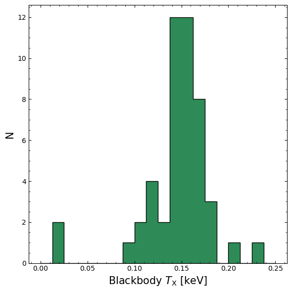
Power-law index#
We repeat the same exercise as in the last section, this time for the power-law index parameter.
Unfortunately, it’s a little harder to define an ‘unphysical’ index value than it was to define an unphysical temperature.
The maximum value of an XSPEC power law photon index (by default) is 10. If a value is in that territory, it’s usually (though not guaranteed to be) the product of a bad fit, so we exclude any rows where the index is \(>9.5\).
We also exclude rows where either of the power-law index uncertainties are negative, or where the uncertainty was flagged as potentially bad at the fitting stage:
res_plind_cut = rass_results.copy()

sel_good = (res_plind_cut["powerlaw_PhoIndex"] < 9.5).values

sel_err_posi = (
    res_plind_cut[["powerlaw_PhoIndex_err-", "powerlaw_PhoIndex_err+"]] > 0
).values.all(axis=1)

res_plind_cut = res_plind_cut[sel_good & sel_err_posi]

res_plind_cut = res_plind_cut[res_plind_cut["powerlaw_PhoIndex_good_err"]]

res_plind_cut.info()
<class 'pandas.DataFrame'>
Index: 65 entries, CARMENES-2 to CARMENES-749
Data columns (total 24 columns):
 #   Column                         Non-Null Count  Dtype
---  ------                         --------------  -----
 0   Karmn                          65 non-null     str
 1   Name                           65 non-null     str
 2   bbody_kT                       65 non-null     float64
 3   bbody_kT_err-                  65 non-null     float64
 4   bbody_kT_err+                  65 non-null     float64
 5   bbody_kT_good_err              65 non-null     bool
 6   bbody_norm                     65 non-null     float64
 7   bbody_norm_err-                65 non-null     float64
 8   bbody_norm_err+                65 non-null     float64
 9   bbody_norm_good_err            65 non-null     bool
 10  powerlaw_PhoIndex              65 non-null     float64
 11  powerlaw_PhoIndex_err-         65 non-null     float64
 12  powerlaw_PhoIndex_err+         65 non-null     float64
 13  powerlaw_PhoIndex_good_err     65 non-null     bool
 14  powerlaw_norm                  65 non-null     float64
 15  powerlaw_norm_err-             65 non-null     float64
 16  powerlaw_norm_err+             65 non-null     float64
 17  powerlaw_norm_good_err         65 non-null     bool
 18  bbody_0.5-2.0keV_flux          65 non-null     float64
 19  bbody_0.5-2.0keV_flux_err-     65 non-null     float64
 20  bbody_0.5-2.0keV_flux_err+     65 non-null     float64
 21  powerlaw_0.5-2.0keV_flux       65 non-null     float64
 22  powerlaw_0.5-2.0keV_flux_err-  65 non-null     float64
 23  powerlaw_0.5-2.0keV_flux_err+  65 non-null     float64
dtypes: bool(4), float64(18), str(2)
memory usage: 13.1 KB
Finally, we make the histogram:
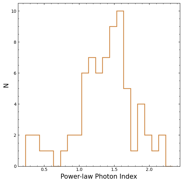
About this notebook#
Author: David Turner, HEASARC Staff Scientist
Author: Mike Corcoran, Associate Research Professor
Updated On: 2026-03-12
Additional Resources#
Support: HEASARC Helpdesk
Acknowledgements#
References#
Alonso-Floriano F. J., Morales J. C., Caballero J. A., Montes D. et al. (2015) - CARMENES input catalogue of M dwarfs. I. Low-resolution spectroscopy with CAFOS
Boller T., Freyberg M.J., Trümper J. et al. (2016) - Second ROSAT all-sky survey (2RXS) source catalogue
The VizieR service DOI: 10.26093/cds/vizier
Ginsburg, Sipőcz, Brasseur et al. (2019) - astroquery: An Astronomical Web-querying Package in Python
Belloni T., Hasinger G., Izzo C. (1994) - Procedures for the interactive analysis of point sources from the ROSAT XRT/PSPC all-sky survey
Caramazza M., Stelzer B., Magaudda E., Raetz St., Güdel M., Orlando S., Poppenhäger K. (2023) - Complete X-ray census of M dwarfs in the solar neighborhood. I. GJ 745 AB: Coronal-hole stars in the 10 pc sample