Using archived and newly generated RXTE light curves#
Learning Goals#
By the end of this tutorial, you will:
Know how to find and use observation tables hosted by HEASARC.
Be able to search for RXTE observations of a named source.
Understand how to access RXTE light curves stored in the HEASARC AWS S3 bucket.
Be capable of downloading and visualizing retrieved light curves.
Know how to generate new RXTE-PCA light curves with:
Custom energy bounds.
Higher temporal resolution than archived products.
Use ‘Continuous Wavelet Transform’ (CWT) peak finding to identify possible bursts.
Introduction#
This notebook is intended to demonstrate how you can use Rossi Timing X-ray Explorer (RXTE) data to examine the temporal variation of a source’s X-ray emission across a wide energy range. We start by identifying and exploring archived RXTE light curves for our source of interest and move on to generating new light curves from raw RXTE Proportional Counter Array (PCA) data.
RXTE was a high-energy mission that provided very high temporal resolution, moderate spectral resolution, observations across a wide energy band (~2–250 keV).
The satellite hosted three instruments:
PCA - Proportional Counter Array; a set of five co-aligned proportional counter units (PCU), sensitive in the 2–60 keV energy band. Collimated ~1 degree full-width half-maximum (FWHM) field-of-view (FoV).
HEXTE - High-Energy X-ray Timing Experiment; a pair of scintillation-counter clusters, sensitive in the 15–250 keV energy band. Collimated ~1 degree FWHM FoV.
ASM - All Sky Monitor; a set of three coded-mask instruments that covered a significant fraction of the sky with each observation (each camera had a 6 x 90 degree FoV). Sensitive in the 2–12 keV energy band.
The PCA and HEXTE instruments had maximum temporal resolutions of \(1 \mu \rm{s}\) and \(8 \mu \rm{s}\) respectively.
Our demonstration is only going to use data from the PCA and HEXTE instruments, and we will only generate new light curves from the PCA instrument.
Though neither PCA nor HEXTE had any imaging capability (they collected photons from their whole FoV without any further spatial information), their time resolution was such that they were very well suited to observations of pulsars; rotating neutron stars with high-energy emission that can vary on the millisecond scale.
We’re going to use a particularly notable pulsar in a low-mass X-ray binary (LMXB) system discovered using RXTE as the subject of our demonstration, ‘IGR J17480–2446’ or ‘T5X2’.
Though it actually rotates quite slowly for a pulsar (“only” ~11 times per second), it displays a number of very interesting behaviors; these include ‘bursts’ of emission caused by infalling gas from its binary companion, and X-ray emission caused by sustained thermonuclear reactions from a large build-up of material possible because of the high accretion rate from its companion.
This behavior had been predicted and modeled, but the first real example was identified in RXTE observations of T5X2, see M. Linares et al. (2012) for full analysis and results.
Inputs#
The name of the source we’ve chosen for the demonstration; IGR J17480–2446 or T5X2.
Outputs#
Visualizations of archived RXTE-PCA and HEXTE light curves.
Newly generated RXTE-PCA light curves within a custom energy band.
Newly generated RXTE-PCA light curves with a higher time resolution than the archived data products.
Runtime#
As of 21st January 2026, this notebook takes ~25 minutes to run to completion on Fornax, using the ‘small’ server with 8GB RAM / 2 cores.
Imports & Environments#
import contextlib
import glob
import multiprocessing as mp
import os
from pprint import pprint
from typing import List, Tuple, Union

import heasoftpy as hsp
import matplotlib.dates as mdates
import matplotlib.pyplot as plt
import numpy as np
import pandas as pd
from astropy.coordinates import SkyCoord
from astropy.io import fits
from astropy.table import unique
from astropy.time import Time
from astropy.units import Quantity
from astroquery.heasarc import Heasarc
from matplotlib import cm
from matplotlib.colors import Normalize
from matplotlib.ticker import FuncFormatter
from s3fs import S3FileSystem
from scipy.signal import find_peaks_cwt
from xga.products import AggregateLightCurve, LightCurve
/opt/envs/heasoft/lib/python3.12/site-packages/xga/utils.py:39: DeprecationWarning: The XGA 'find_all_wcs' function should be imported from imagetools.misc, in the future it will be removed from utils.
  warn(message, DeprecationWarning)
/opt/envs/heasoft/lib/python3.12/site-packages/xga/utils.py:619: UserWarning: SAS_DIR environment variable is not set, unable to verify SAS is present on system, as such all functions in xga.sas will not work.
  warn("SAS_DIR environment variable is not set, unable to verify SAS is present on system, as such "
/opt/envs/heasoft/lib/python3.12/site-packages/xga/__init__.py:6: UserWarning: This is the first time you've used XGA; to use most functionality you will need to configure /home/jovyan/.config/xga/xga.cfg to match your setup, though you can use product classes regardless.
  from .utils import xga_conf, CENSUS, OUTPUT, NUM_CORES, XGA_EXTRACT, BASE_XSPEC_SCRIPT, CROSS_ARF_XSPEC_SCRIPT, \
/opt/envs/heasoft/lib/python3.12/site-packages/xga/products/relation.py:12: DeprecationWarning: `scipy.odr` is deprecated as of version 1.17.0 and will be removed in SciPy 1.19.0. Please use `https://pypi.org/project/odrpack/` instead.
  import scipy.odr as odr
Global Setup#
Functions#
Constants#
Configuration#
1. Finding the data#
To identify relevant RXTE data, we could use Xamin, the HEASARC web portal, the Virtual Observatory (VO) python client pyvo, or the Astroquery module (our choice for this demonstration).
Using Astroquery to find the RXTE observation summary (master) table#
Using the Heasarc object from Astroquery, we can easily search through all of HEASARC’s catalog holdings. In this
case we need to find what we refer to as a ‘master’ catalog/table, which summarizes all RXTE observations present in
our archive. We can do this by passing the master=True keyword argument to the list_catalogs method.
table_name = Heasarc.list_catalogs(keywords="xte", master=True)[0]["name"]
table_name
np.str_('xtemaster')
Identifying RXTE observations of IGR J17480–2446/T5X2#
Now that we have identified the HEASARC table that contains information on RXTE pointings, we’re going to search it for observations of T5X2.
For convenience, we pull the coordinate of T5X2/IGR J17480–2446 from the Strasbourg astronomical Data Center (CDS) name
resolver functionality built into Astropy’s SkyCoord class. A constant containing the name of the target was created in
the ‘Global Setup: Constants’ section of this notebook:
SRC_NAME
'IGR J17480–2446'
Using the SkyCoord class, we can fetch the coordinates for our target:
# Get the coordinate for our source
rel_coord = SkyCoord.from_name(SRC_NAME)
# Turn it into a straight Astropy quantity, which will be useful later
rel_coord_quan = Quantity([rel_coord.ra, rel_coord.dec])
rel_coord
<SkyCoord (ICRS): (ra, dec) in deg
    (267.0201292, -24.7802417)>
Hint
Each HEASARC catalog has its own default search radius, which you can retrieve
using Heasarc.get_default_radius(catalog_name) - you should carefully consider the
search radius you use for your own science case!
Then we can use the query_region method of Heasarc to search for relevant RXTE observations:
all_obs = Heasarc.query_region(rel_coord, catalog=table_name)
all_obs
| obsid | prnb | status | pi_lname | pi_fname | target_name | ra | dec | time | duration | exposure | __row |
|---|---|---|---|---|---|---|---|---|---|---|---|
| deg | deg | d | s | s | |||||||
| object | int32 | object | object | object | object | float64 | float64 | float64 | float64 | float64 | object |
| 93055 | accepted | ALTAMIRANO | DIEGO | EXO1745-248 | 267.2333 | -24.8950 | -- | -- | -- | 70727 | |
| 50054-06-01-01 | 50054 | archived | ZHANG | WILLIAM | EXO_1745-248 | 267.0225 | -24.7819 | 51749.63341 | 5820 | 2429 | 71046 |
| 50054-06-01-00 | 50054 | archived | ZHANG | WILLIAM | EXO_1745-248 | 267.0225 | -24.7819 | 51746.43203 | 6047 | 3434 | 71047 |
| 50138-03-01-00 | 50138 | archived | SWANK | JEAN | EXO_1745-248 | 267.0225 | -24.7819 | 51738.18831 | 3260 | 1680 | 71048 |
| 50138-03-01-01 | 50138 | archived | SWANK | JEAN | EXO_1745-248 | 267.0225 | -24.7819 | 51738.73752 | 3217 | 1735 | 71049 |
| 50138-03-02-00 | 50138 | archived | SWANK | JEAN | EXO_1745-248 | 267.0225 | -24.7819 | 51740.0494 | 2940 | 1064 | 71050 |
| 50138-03-02-01 | 50138 | archived | SWANK | JEAN | EXO_1745-248 | 267.0225 | -24.7819 | 51740.11606 | 541 | -- | 71051 |
| 50138-03-03-00 | 50138 | archived | SWANK | JEAN | EXO_1745-248 | 267.0225 | -24.7819 | 51741.44572 | 5237 | 3378 | 71052 |
| 50138-03-04-00 | 50138 | archived | SWANK | JEAN | EXO_1745-248 | 267.0225 | -24.7819 | 51742.50841 | 4596 | 3477 | 71053 |
| ... | ... | ... | ... | ... | ... | ... | ... | ... | ... | ... | ... |
| 96316-01-16-00 | 96316 | archived | ALTAMIRANO | DIEGO | TERZAN_5 | 267.0208 | -24.7800 | 55684.96769 | 2770 | 1917 | 71196 |
| 96316-01-17-00 | 96316 | archived | ALTAMIRANO | DIEGO | TERZAN_5 | 267.0208 | -24.7800 | 55691.58411 | 4860 | 1667 | 71197 |
| 96316-01-18-00 | 96316 | archived | ALTAMIRANO | DIEGO | TERZAN_5 | 267.0208 | -24.7800 | 55697.92324 | 4419 | 2101 | 71198 |
| 96316-01-19-00 | 96316 | archived | ALTAMIRANO | DIEGO | TERZAN_5 | 267.0208 | -24.7800 | 55704.84321 | 4554 | 2130 | 71199 |
| 96316-01-20-00 | 96316 | archived | ALTAMIRANO | DIEGO | TERZAN_5 | 267.0208 | -24.7800 | 55711.75772 | 3631 | 1622 | 71200 |
| 96316-01-21-00 | 96316 | archived | ALTAMIRANO | DIEGO | TERZAN_5 | 267.0208 | -24.7800 | 55718.35848 | 4744 | 2013 | 71201 |
| 96316-01-22-00 | 96316 | archived | ALTAMIRANO | DIEGO | TERZAN_5 | 267.0208 | -24.7800 | 55725.37816 | 3388 | 2213 | 71202 |
| 96316-01-23-00 | 96316 | archived | ALTAMIRANO | DIEGO | TERZAN_5 | 267.0208 | -24.7800 | 55731.20844 | 4067 | 2078 | 71203 |
| 96316-01-24-00 | 96316 | archived | ALTAMIRANO | DIEGO | TERZAN_5 | 267.0208 | -24.7800 | 55739.64314 | 4437 | 1933 | 71204 |
We can immediately see that the first entry in the all_obs table does not have
an ObsID, and is also missing other crucial information such as when the observation
was taken, and how long the exposure was. This is because a proposal was accepted, but
the data were never taken. In this case it’s likely because the proposal was for a
target of opportunity (ToO), and the trigger conditions were never met.
All that said, we should filter our table of observations to ensure that only real observations are included. The easiest way to do that is probably to require that the exposure time entry is greater than zero:
valid_obs = all_obs[all_obs["exposure"] > 0]
valid_obs
| obsid | prnb | status | pi_lname | pi_fname | target_name | ra | dec | time | duration | exposure | __row |
|---|---|---|---|---|---|---|---|---|---|---|---|
| deg | deg | d | s | s | |||||||
| object | int32 | object | object | object | object | float64 | float64 | float64 | float64 | float64 | object |
| 50054-06-01-01 | 50054 | archived | ZHANG | WILLIAM | EXO_1745-248 | 267.0225 | -24.7819 | 51749.63341 | 5820 | 2429 | 71046 |
| 50054-06-01-00 | 50054 | archived | ZHANG | WILLIAM | EXO_1745-248 | 267.0225 | -24.7819 | 51746.43203 | 6047 | 3434 | 71047 |
| 50138-03-01-00 | 50138 | archived | SWANK | JEAN | EXO_1745-248 | 267.0225 | -24.7819 | 51738.18831 | 3260 | 1680 | 71048 |
| 50138-03-01-01 | 50138 | archived | SWANK | JEAN | EXO_1745-248 | 267.0225 | -24.7819 | 51738.73752 | 3217 | 1735 | 71049 |
| 50138-03-02-00 | 50138 | archived | SWANK | JEAN | EXO_1745-248 | 267.0225 | -24.7819 | 51740.0494 | 2940 | 1064 | 71050 |
| 50138-03-03-00 | 50138 | archived | SWANK | JEAN | EXO_1745-248 | 267.0225 | -24.7819 | 51741.44572 | 5237 | 3378 | 71052 |
| 50138-03-04-00 | 50138 | archived | SWANK | JEAN | EXO_1745-248 | 267.0225 | -24.7819 | 51742.50841 | 4596 | 3477 | 71053 |
| 50138-03-05-00 | 50138 | archived | SWANK | JEAN | EXO_1745-248 | 267.0225 | -24.7819 | 51743.57614 | 4176 | 3038 | 71054 |
| 50054-06-02-01 | 50054 | archived | ZHANG | WILLIAM | EXO_1745-248 | 267.0225 | -24.7819 | 51756.25972 | 4793 | 3539 | 71055 |
| ... | ... | ... | ... | ... | ... | ... | ... | ... | ... | ... | ... |
| 96316-01-16-00 | 96316 | archived | ALTAMIRANO | DIEGO | TERZAN_5 | 267.0208 | -24.7800 | 55684.96769 | 2770 | 1917 | 71196 |
| 96316-01-17-00 | 96316 | archived | ALTAMIRANO | DIEGO | TERZAN_5 | 267.0208 | -24.7800 | 55691.58411 | 4860 | 1667 | 71197 |
| 96316-01-18-00 | 96316 | archived | ALTAMIRANO | DIEGO | TERZAN_5 | 267.0208 | -24.7800 | 55697.92324 | 4419 | 2101 | 71198 |
| 96316-01-19-00 | 96316 | archived | ALTAMIRANO | DIEGO | TERZAN_5 | 267.0208 | -24.7800 | 55704.84321 | 4554 | 2130 | 71199 |
| 96316-01-20-00 | 96316 | archived | ALTAMIRANO | DIEGO | TERZAN_5 | 267.0208 | -24.7800 | 55711.75772 | 3631 | 1622 | 71200 |
| 96316-01-21-00 | 96316 | archived | ALTAMIRANO | DIEGO | TERZAN_5 | 267.0208 | -24.7800 | 55718.35848 | 4744 | 2013 | 71201 |
| 96316-01-22-00 | 96316 | archived | ALTAMIRANO | DIEGO | TERZAN_5 | 267.0208 | -24.7800 | 55725.37816 | 3388 | 2213 | 71202 |
| 96316-01-23-00 | 96316 | archived | ALTAMIRANO | DIEGO | TERZAN_5 | 267.0208 | -24.7800 | 55731.20844 | 4067 | 2078 | 71203 |
| 96316-01-24-00 | 96316 | archived | ALTAMIRANO | DIEGO | TERZAN_5 | 267.0208 | -24.7800 | 55739.64314 | 4437 | 1933 | 71204 |
Then, by converting the ‘time’ column of the valid observations table into an Astropy
Time object, and using the min() and max() methods, we can see that the
observations we’ve selected come from a period of over 10 years.
valid_obs_times = Time(valid_obs["time"], format="mjd")
valid_obs_datetimes = valid_obs_times.to_datetime()
print(valid_obs_datetimes.min())
print(valid_obs_datetimes.max())
2000-07-13 04:31:09.984000
2011-11-19 14:08:29.472000
To reduce the run time of this demonstration, we’ll select observations taken before the 19th of October 2010. There are a significant number of observations taken after this date, but the light curves are not as featureful and interesting as those taken before.
cut_valid_obs = valid_obs[valid_obs_times < Time("2010-10-19")]
rel_obsids = np.array(cut_valid_obs["obsid"])
print(len(rel_obsids))
62
Constructing an ADQL query [advanced alternative]#
Alternatively, if you wished to place extra constraints on the search, you could use the more complex but more powerful
query_tap method to pass a full Astronomical Data Query Language (ADQL) query. This demonstration runs the same
spatial query as before but also includes a stringent exposure time requirement; you might do this to try and only
select the highest signal-to-noise observations.
Note that we call the to_table method on the result of the query to convert the result into an Astropy table, which
is the form required to pass to the locate_data method (see the next section).
query = (
    "SELECT * "
    "from {c} as cat "
    "where contains(point('ICRS',cat.ra,cat.dec), circle('ICRS',{ra},{dec},0.0033))=1 "
    "and cat.exposure > 0".format(
        ra=rel_coord.ra.value, dec=rel_coord.dec.value, c=table_name
    )
)

alt_obs = Heasarc.query_tap(query).to_table()
alt_obs
| __row | pi_lname | pi_fname | pi_no | prnb | cycle | subject_category | target_name | time_awarded | ra | dec | priority | tar_no | obsid | time | duration | exposure | status | scheduled_date | observed_date | processed_date | archived_date | hexte_anglea | hexte_angleb | hexte_dwella | hexte_dwellb | hexte_energya | hexte_energyb | hexte_modea | hexte_modeb | pca_config1 | pca_config2 | pca_config3 | pca_config4 | pca_config5 | pca_config6 | lii | bii | __x_ra_dec | __y_ra_dec | __z_ra_dec |
|---|---|---|---|---|---|---|---|---|---|---|---|---|---|---|---|---|---|---|---|---|---|---|---|---|---|---|---|---|---|---|---|---|---|---|---|---|---|---|---|---|
| s | deg | deg | d | s | s | d | d | d | d | deg | deg | |||||||||||||||||||||||||||||
| object | object | object | int32 | int32 | int16 | object | object | float64 | float64 | float64 | int16 | int16 | object | float64 | float64 | float64 | object | float64 | float64 | int32 | int32 | object | object | object | object | object | object | object | object | object | object | object | object | object | object | float64 | float64 | float64 | float64 | float64 |
| 71046 | ZHANG | WILLIAM | 164 | 50054 | 5 | LMXB | EXO_1745-248 | 200000.0 | 267.0225 | -24.7819 | 1 | 6 | 50054-06-01-01 | 51749.63341 | 5820 | 2429 | archived | 51749.63341 | 51749.63341 | -- | 52129 | DEFAULT | DEFAULT | DEFAULT | DEFAULT | DEFAULT | DEFAULT | E_8US_256_DX0F | E_8US_256_DX0F | STANDARD1 | STANDARD2 | E_125US_64M_0_1S | TLA_1S_10_249_1S_10000_F | CB_125US_1M_0_249_H | IDLE | 3.8381 | 1.6836 | -0.906683970297968 | -0.0471604275070132 | -0.419165924285443 |
| 71047 | ZHANG | WILLIAM | 164 | 50054 | 5 | LMXB | EXO_1745-248 | 200000.0 | 267.0225 | -24.7819 | 1 | 6 | 50054-06-01-00 | 51746.43203 | 6047 | 3434 | archived | 51746.43203 | 51746.43203 | -- | 52122 | DEFAULT | DEFAULT | DEFAULT | DEFAULT | DEFAULT | DEFAULT | E_8US_256_DX0F | E_8US_256_DX0F | STANDARD1 | STANDARD2 | E_125US_64M_0_1S | TLA_1S_10_249_1S_10000_F | CB_125US_1M_0_249_H | IDLE | 3.8381 | 1.6836 | -0.906683970297968 | -0.0471604275070132 | -0.419165924285443 |
| 71048 | SWANK | JEAN | 168 | 50138 | 5 | OTHER | EXO_1745-248 | 15000.0 | 267.0225 | -24.7819 | 1 | 3 | 50138-03-01-00 | 51738.18831 | 3260 | 1680 | archived | 51738.18831 | 51738.18831 | -- | 52122 | DEFAULT | DEFAULT | DEFAULT | DEFAULT | DEFAULT | DEFAULT | E_8US_256_DX1F | E_8US_256_DX1F | STANDARD1 | STANDARD2 | TLA_1S_10_249_1S_5000_F | CB_125US_1M_0_249_H | CB_8MS_64M_0_249_H | E_125US_64M_0_1S | 3.8381 | 1.6836 | -0.906683970297968 | -0.0471604275070132 | -0.419165924285443 |
| 71049 | SWANK | JEAN | 168 | 50138 | 5 | OTHER | EXO_1745-248 | 15000.0 | 267.0225 | -24.7819 | 1 | 3 | 50138-03-01-01 | 51738.73752 | 3217 | 1735 | archived | 51738.73752 | 51738.73752 | -- | 52122 | DEFAULT | DEFAULT | DEFAULT | DEFAULT | DEFAULT | DEFAULT | E_8US_256_DX1F | E_8US_256_DX1F | STANDARD1 | STANDARD2 | TLA_1S_10_249_1S_5000_F | CB_125US_1M_0_249_H | CB_8MS_64M_0_249_H | E_125US_64M_0_1S | 3.8381 | 1.6836 | -0.906683970297968 | -0.0471604275070132 | -0.419165924285443 |
| 71050 | SWANK | JEAN | 168 | 50138 | 5 | OTHER | EXO_1745-248 | 15000.0 | 267.0225 | -24.7819 | 1 | 3 | 50138-03-02-00 | 51740.0494 | 2940 | 1064 | archived | 51740.0494 | 51740.0494 | -- | 52122 | DEFAULT | DEFAULT | DEFAULT | DEFAULT | DEFAULT | DEFAULT | E_8US_256_DX1F | E_8US_256_DX1F | STANDARD1 | STANDARD2 | TLA_1S_10_249_1S_5000_F | CB_125US_1M_0_249_H | CB_8MS_64M_0_249_H | E_125US_64M_0_1S | 3.8381 | 1.6836 | -0.906683970297968 | -0.0471604275070132 | -0.419165924285443 |
| 71052 | SWANK | JEAN | 168 | 50138 | 5 | OTHER | EXO_1745-248 | 15000.0 | 267.0225 | -24.7819 | 1 | 3 | 50138-03-03-00 | 51741.44572 | 5237 | 3378 | archived | 51741.44572 | 51741.44572 | -- | 52122 | DEFAULT | DEFAULT | DEFAULT | DEFAULT | DEFAULT | DEFAULT | E_8US_256_DX1F | E_8US_256_DX1F | STANDARD1 | STANDARD2 | TLA_1S_10_249_1S_5000_F | CB_125US_1M_0_249_H | CB_8MS_64M_0_249_H | E_125US_64M_0_1S | 3.8381 | 1.6836 | -0.906683970297968 | -0.0471604275070132 | -0.419165924285443 |
| 71053 | SWANK | JEAN | 168 | 50138 | 5 | OTHER | EXO_1745-248 | 15000.0 | 267.0225 | -24.7819 | 1 | 3 | 50138-03-04-00 | 51742.50841 | 4596 | 3477 | archived | 51742.50841 | 51742.50841 | -- | 52122 | DEFAULT | DEFAULT | DEFAULT | DEFAULT | DEFAULT | DEFAULT | E_8US_256_DX1F | E_8US_256_DX1F | STANDARD1 | STANDARD2 | TLA_1S_10_249_1S_5000_F | CB_125US_1M_0_249_H | CB_8MS_64M_0_249_H | E_125US_64M_0_1S | 3.8381 | 1.6836 | -0.906683970297968 | -0.0471604275070132 | -0.419165924285443 |
| 71054 | SWANK | JEAN | 168 | 50138 | 5 | OTHER | EXO_1745-248 | 15000.0 | 267.0225 | -24.7819 | 1 | 3 | 50138-03-05-00 | 51743.57614 | 4176 | 3038 | archived | 51743.57614 | 51743.57614 | -- | 52122 | DEFAULT | DEFAULT | DEFAULT | DEFAULT | DEFAULT | DEFAULT | E_8US_256_DX1F | E_8US_256_DX1F | STANDARD1 | STANDARD2 | TLA_1S_10_249_1S_5000_F | CB_125US_1M_0_249_H | CB_8MS_64M_0_249_H | E_125US_64M_0_1S | 3.8381 | 1.6836 | -0.906683970297968 | -0.0471604275070132 | -0.419165924285443 |
| 71055 | ZHANG | WILLIAM | 164 | 50054 | 5 | LMXB | EXO_1745-248 | 200000.0 | 267.0225 | -24.7819 | 1 | 6 | 50054-06-02-01 | 51756.25972 | 4793 | 3539 | archived | 51756.25972 | 51756.25972 | -- | 52151 | DEFAULT | DEFAULT | DEFAULT | DEFAULT | DEFAULT | DEFAULT | E_8US_256_DX0F | E_8US_256_DX0F | STANDARD1 | STANDARD2 | E_125US_64M_0_1S | TLA_1S_10_249_1S_10000_F | CB_125US_1M_0_249_H | IDLE | 3.8381 | 1.6836 | -0.906684262535712 | -0.0471604427075212 | -0.419165290444834 |
| ... | ... | ... | ... | ... | ... | ... | ... | ... | ... | ... | ... | ... | ... | ... | ... | ... | ... | ... | ... | ... | ... | ... | ... | ... | ... | ... | ... | ... | ... | ... | ... | ... | ... | ... | ... | ... | ... | ... | ... | ... |
| 71196 | ALTAMIRANO | DIEGO | 530 | 96316 | 15 | LMXB | TERZAN_5 | 1920.0 | 267.0208 | -24.7800 | 0 | 1 | 96316-01-16-00 | 55684.96769 | 2770 | 1917 | archived | 55684.96769 | 55684.96769 | 55693 | -- | DEFAULT | DEFAULT | DEFAULT | DEFAULT | DEFAULT | DEFAULT | E_8us_256_DX1F | E_8us_256_DX1F | GOODXENON1_2S | GOODXENON2_2S | D_1US_0_249_1024_64S_F | STANDARD1B | STANDARD2F | D_1US_0_249_1024_64S_F | 3.8389 | 1.6859 | -0.906696760092206 | -0.0471877504630087 | -0.419135182780613 |
| 71197 | ALTAMIRANO | DIEGO | 530 | 96316 | 15 | LMXB | TERZAN_5 | 1670.0 | 267.0208 | -24.7800 | 0 | 1 | 96316-01-17-00 | 55691.58411 | 4860 | 1667 | archived | 55691.58411 | 55691.58411 | 55699 | -- | DEFAULT | DEFAULT | DEFAULT | DEFAULT | DEFAULT | DEFAULT | E_8us_256_DX1F | E_8us_256_DX1F | GOODXENON1_2S | GOODXENON2_2S | D_1US_0_249_1024_64S_F | STANDARD1B | STANDARD2F | D_1US_0_249_1024_64S_F | 3.8389 | 1.6859 | -0.906696760092206 | -0.0471877504630087 | -0.419135182780613 |
| 71198 | ALTAMIRANO | DIEGO | 530 | 96316 | 15 | LMXB | TERZAN_5 | 2100.0 | 267.0208 | -24.7800 | 0 | 1 | 96316-01-18-00 | 55697.92324 | 4419 | 2101 | archived | 55697.92324 | 55697.92324 | 55705 | -- | DEFAULT | DEFAULT | DEFAULT | DEFAULT | DEFAULT | DEFAULT | E_8us_256_DX1F | E_8us_256_DX1F | GOODXENON1_2S | GOODXENON2_2S | D_1US_0_249_1024_64S_F | STANDARD1B | STANDARD2F | D_1US_0_249_1024_64S_F | 3.8389 | 1.6859 | -0.906696760092206 | -0.0471877504630087 | -0.419135182780613 |
| 71199 | ALTAMIRANO | DIEGO | 530 | 96316 | 15 | LMXB | TERZAN_5 | 2130.0 | 267.0208 | -24.7800 | 0 | 1 | 96316-01-19-00 | 55704.84321 | 4554 | 2130 | archived | 55704.84321 | 55704.84321 | 55712 | -- | DEFAULT | DEFAULT | DEFAULT | DEFAULT | DEFAULT | DEFAULT | E_8us_256_DX1F | E_8us_256_DX1F | GOODXENON1_2S | GOODXENON2_2S | D_1US_0_249_1024_64S_F | STANDARD1B | STANDARD2F | D_1US_0_249_1024_64S_F | 3.8389 | 1.6859 | -0.906696760092206 | -0.0471877504630087 | -0.419135182780613 |
| 71200 | ALTAMIRANO | DIEGO | 530 | 96316 | 15 | LMXB | TERZAN_5 | 1620.0 | 267.0208 | -24.7800 | 0 | 1 | 96316-01-20-00 | 55711.75772 | 3631 | 1622 | archived | 55711.75772 | 55711.75772 | 55719 | -- | DEFAULT | DEFAULT | DEFAULT | DEFAULT | DEFAULT | DEFAULT | E_8us_256_DX1F | E_8us_256_DX1F | GOODXENON1_2S | GOODXENON2_2S | D_1US_0_249_1024_64S_F | STANDARD1B | STANDARD2F | D_1US_0_249_1024_64S_F | 3.8389 | 1.6859 | -0.906696760092206 | -0.0471877504630087 | -0.419135182780613 |
| 71201 | ALTAMIRANO | DIEGO | 530 | 96316 | 15 | LMXB | TERZAN_5 | 2010.0 | 267.0208 | -24.7800 | 0 | 1 | 96316-01-21-00 | 55718.35848 | 4744 | 2013 | archived | 55718.35848 | 55718.35848 | 55726 | -- | DEFAULT | DEFAULT | DEFAULT | DEFAULT | DEFAULT | DEFAULT | E_8us_256_DX1F | E_8us_256_DX1F | GOODXENON1_2S | GOODXENON2_2S | D_1US_0_249_1024_64S_F | STANDARD1B | STANDARD2F | D_1US_0_249_1024_64S_F | 3.8389 | 1.6859 | -0.906696760092206 | -0.0471877504630087 | -0.419135182780613 |
| 71202 | ALTAMIRANO | DIEGO | 530 | 96316 | 15 | LMXB | TERZAN_5 | 2210.0 | 267.0208 | -24.7800 | 0 | 1 | 96316-01-22-00 | 55725.37816 | 3388 | 2213 | archived | 55725.37816 | 55725.37816 | 55733 | -- | DEFAULT | DEFAULT | DEFAULT | DEFAULT | DEFAULT | DEFAULT | E_8us_256_DX1F | E_8us_256_DX1F | GOODXENON1_2S | GOODXENON2_2S | D_1US_0_249_1024_64S_F | STANDARD1B | STANDARD2F | D_1US_0_249_1024_64S_F | 3.8389 | 1.6859 | -0.906696760092206 | -0.0471877504630087 | -0.419135182780613 |
| 71203 | ALTAMIRANO | DIEGO | 530 | 96316 | 15 | LMXB | TERZAN_5 | 2080.0 | 267.0208 | -24.7800 | 0 | 1 | 96316-01-23-00 | 55731.20844 | 4067 | 2078 | archived | 55731.20844 | 55731.20844 | 55739 | -- | DEFAULT | DEFAULT | DEFAULT | DEFAULT | DEFAULT | DEFAULT | E_8us_256_DX1F | E_8us_256_DX1F | GOODXENON1_2S | GOODXENON2_2S | D_1US_0_249_1024_64S_F | STANDARD1B | STANDARD2F | D_1US_0_249_1024_64S_F | 3.8389 | 1.6859 | -0.906696760092206 | -0.0471877504630087 | -0.419135182780613 |
| 71204 | ALTAMIRANO | DIEGO | 530 | 96316 | 15 | LMXB | TERZAN_5 | 1930.0 | 267.0208 | -24.7800 | 0 | 1 | 96316-01-24-00 | 55739.64314 | 4437 | 1933 | archived | 55739.64314 | 55739.64314 | 55749 | -- | DEFAULT | DEFAULT | DEFAULT | DEFAULT | DEFAULT | DEFAULT | E_8us_256_DX1F | E_8us_256_DX1F | GOODXENON1_2S | GOODXENON2_2S | D_1US_0_249_1024_64S_F | STANDARD1B | STANDARD2F | D_1US_0_249_1024_64S_F | 3.8389 | 1.6859 | -0.906696760092206 | -0.0471877504630087 | -0.419135182780613 |
Using Astroquery to fetch datalinks to RXTE datasets#
We’ve already figured out which HEASARC table to pull RXTE observation information from, and then used that table to identify specific observations that might be relevant to our target source (T5X2). Our next step is to pinpoint the exact locations of each observation’s data files.
Just as in the last two steps, we’re going to make use of Astroquery. The difference is, rather than dealing with tables of observations, we now need to construct ‘datalinks’ to places where specific files for each observation are stored. In this demonstration we’re going to pull data from the HEASARC ‘S3 bucket’, an Amazon-hosted open-source dataset containing all of HEASARC’s data holdings.
For our use case, we’re going to exclude any data links that point to data directories containing non-pointing portions of RXTE observations; in practise that means data collected during slewing before and after the observation of our target. Slewing data can be more difficult to work with, so for this demonstration we’re going to ignore it. The data links tell us which directories contain such data through the final character of the directory name:
A - Slewing data from before the observation.
Z - Slewing data from after the observation.
S - Data taken in scan mode.
R - Data taken in a raster grid mode.
See also
This HEASARC page details the standard contents of RXTE observation directories, as well as the standard names of files and sub-directories. Section 3.3 explains the meanings of the characters we discussed above.
data_links = Heasarc.locate_data(cut_valid_obs, "xtemaster")

# Drop rows with duplicate AWS links
data_links = unique(data_links, keys="aws")

# Drop rows that represent directories of slewing, scanning, or raster scanning
#  observation data
non_pnting = (
    np.char.endswith(data_links["aws"].value[..., None], ["Z/", "A/", "S/", "R/"]).sum(
        axis=1
    )
    == 0
)
data_links = data_links[non_pnting]

data_links[-10:]
| ID | access_url | sciserver | aws | content_length | error_message |
|---|---|---|---|---|---|
| byte | |||||
| object | object | str50 | str63 | int64 | object |
| ivo://nasa.heasarc/xtemaster?71049 | https://heasarc.gsfc.nasa.gov/FTP/xte/data/archive/AO5/P50138//50138-03-01-01/ | /FTP/xte/data/archive/AO5/P50138/50138-03-01-01/ | s3://nasa-heasarc/xte/data/archive/AO5/P50138/50138-03-01-01/ | -- | |
| ivo://nasa.heasarc/xtemaster?71050 | https://heasarc.gsfc.nasa.gov/FTP/xte/data/archive/AO5/P50138//50138-03-02-00/ | /FTP/xte/data/archive/AO5/P50138/50138-03-02-00/ | s3://nasa-heasarc/xte/data/archive/AO5/P50138/50138-03-02-00/ | -- | |
| ivo://nasa.heasarc/xtemaster?71052 | https://heasarc.gsfc.nasa.gov/FTP/xte/data/archive/AO5/P50138//50138-03-03-00/ | /FTP/xte/data/archive/AO5/P50138/50138-03-03-00/ | s3://nasa-heasarc/xte/data/archive/AO5/P50138/50138-03-03-00/ | -- | |
| ivo://nasa.heasarc/xtemaster?71053 | https://heasarc.gsfc.nasa.gov/FTP/xte/data/archive/AO5/P50138//50138-03-04-00/ | /FTP/xte/data/archive/AO5/P50138/50138-03-04-00/ | s3://nasa-heasarc/xte/data/archive/AO5/P50138/50138-03-04-00/ | -- | |
| ivo://nasa.heasarc/xtemaster?71054 | https://heasarc.gsfc.nasa.gov/FTP/xte/data/archive/AO5/P50138//50138-03-05-00/ | /FTP/xte/data/archive/AO5/P50138/50138-03-05-00/ | s3://nasa-heasarc/xte/data/archive/AO5/P50138/50138-03-05-00/ | -- | |
| ivo://nasa.heasarc/xtemaster?71048 | https://heasarc.gsfc.nasa.gov/FTP/xte/data/archive/AO5/P50138//50138-03/ | /FTP/xte/data/archive/AO5/P50138/50138-03/ | s3://nasa-heasarc/xte/data/archive/AO5/P50138/50138-03/ | -- | |
| ivo://nasa.heasarc/xtemaster?71147 | https://heasarc.gsfc.nasa.gov/FTP/xte/data/archive/AO7/P70412//70412-01-01-00/ | /FTP/xte/data/archive/AO7/P70412/70412-01-01-00/ | s3://nasa-heasarc/xte/data/archive/AO7/P70412/70412-01-01-00/ | -- | |
| ivo://nasa.heasarc/xtemaster?71082 | https://heasarc.gsfc.nasa.gov/FTP/xte/data/archive/AO7/P70412//70412-01-02-00/ | /FTP/xte/data/archive/AO7/P70412/70412-01-02-00/ | s3://nasa-heasarc/xte/data/archive/AO7/P70412/70412-01-02-00/ | -- | |
| ivo://nasa.heasarc/xtemaster?71081 | https://heasarc.gsfc.nasa.gov/FTP/xte/data/archive/AO7/P70412//70412-01-03-00/ | /FTP/xte/data/archive/AO7/P70412/70412-01-03-00/ | s3://nasa-heasarc/xte/data/archive/AO7/P70412/70412-01-03-00/ | -- | |
| ivo://nasa.heasarc/xtemaster?71081 | https://heasarc.gsfc.nasa.gov/FTP/xte/data/archive/AO7/P70412//70412-01/ | /FTP/xte/data/archive/AO7/P70412/70412-01/ | s3://nasa-heasarc/xte/data/archive/AO7/P70412/70412-01/ | -- |
2. Acquiring the data#
We now know where the relevant RXTE light curves are stored in the HEASARC S3 bucket and will proceed to download them for local use.
The easiest way to download data#
At this point, you may wish to simply download the entire set of files for all the observations you’ve identified.
That is easily achieved using Astroquery, with the download_data method of Heasarc, we just need to pass
the datalinks we found in the previous step.
We demonstrate this approach using the first three entries in the datalinks table, but in the following sections will demonstrate a more complicated, but targeted, approach that will let us download the light curve files only:
Heasarc.download_data(data_links[:3], host="aws", location=ROOT_DATA_DIR)
INFO: Downloading data AWS S3 ... [astroquery.heasarc.core]
INFO: Enabling anonymous cloud data access ... [astroquery.heasarc.core]
INFO: downloading s3://nasa-heasarc/xte/data/archive/AO14/P95437/95437-01-01-00/ [astroquery.heasarc.core]
INFO: downloading s3://nasa-heasarc/xte/data/archive/AO14/P95437/95437-01-02-00/ [astroquery.heasarc.core]
INFO: downloading s3://nasa-heasarc/xte/data/archive/AO14/P95437/95437-01-02-01/ [astroquery.heasarc.core]
Downloading only the archived RXTE light curves#
Rather than downloading all files for all our observations, we will now only fetch those that are directly relevant to what we want to do in this notebook - this method is a little more involved than using Astroquery, but it is more efficient and flexible.
We make use of a Python module called s3fs, which allows us to interact with files stored on Amazon’s S3
platform through Python commands.
We create an S3FileSystem object, which lets us interact with the S3 bucket as if it were a filesystem.
Hint
Note the anon=True argument, as attempting access to the HEASARC S3 bucket will fail without it!
s3 = S3FileSystem(anon=True)
Now we identify the specific files we want to download. The datalink table tells us the AWS S3 ‘path’ (the Uniform Resource Identifier, or URI) to each observation’s data directory, the RXTE documentation tells us that the automatically generated data products are stored in a subdirectory called ‘stdprod’, and the RXTE Guest Observer Facility (GOF) standard product guide shows us that the net light curves are named as:
xp{ObsID}_n2{energy-band}.lc - PCA
xh{ObsID}_n{array-number}{energy-band}.lc - HEXTE
We set up file patterns for the light curves we’re interested in, and then use the expand_path method of
our previously set-up S3 filesystem object to find all the files stored at each data-link’s destination that match the pattern. This is useful because the
RXTE datalinks we found might include sections of a particular observation that do not have standard products
generated, for instance, the slewing periods before/after the telescope was aligned on target.
lc_patts = ["xp*_n2*.lc.gz", "xh*_n0*.lc.gz", "xh*_n1*.lc.gz"]

all_file_patt = [
    os.path.join(base_uri, "stdprod", fp)
    for base_uri in data_links["aws"].value
    for fp in lc_patts
]

val_file_uris = s3.expand_path(all_file_patt)
val_file_uris[:10]
['nasa-heasarc/xte/data/archive/AO14/P95437/95437-01-01-00/stdprod/xp95437010100_n2a.lc.gz',
 'nasa-heasarc/xte/data/archive/AO14/P95437/95437-01-01-00/stdprod/xp95437010100_n2b.lc.gz',
 'nasa-heasarc/xte/data/archive/AO14/P95437/95437-01-01-00/stdprod/xp95437010100_n2c.lc.gz',
 'nasa-heasarc/xte/data/archive/AO14/P95437/95437-01-01-00/stdprod/xp95437010100_n2d.lc.gz',
 'nasa-heasarc/xte/data/archive/AO14/P95437/95437-01-01-00/stdprod/xp95437010100_n2e.lc.gz',
 'nasa-heasarc/xte/data/archive/AO14/P95437/95437-01-02-00/stdprod/xp95437010200_n2a.lc.gz',
 'nasa-heasarc/xte/data/archive/AO14/P95437/95437-01-02-00/stdprod/xp95437010200_n2b.lc.gz',
 'nasa-heasarc/xte/data/archive/AO14/P95437/95437-01-02-00/stdprod/xp95437010200_n2c.lc.gz',
 'nasa-heasarc/xte/data/archive/AO14/P95437/95437-01-02-00/stdprod/xp95437010200_n2d.lc.gz',
 'nasa-heasarc/xte/data/archive/AO14/P95437/95437-01-02-00/stdprod/xp95437010200_n2e.lc.gz']
Now we can just use the get method of our S3 filesystem object to download all the valid light curve files!
lc_file_path = os.path.join(ROOT_DATA_DIR, "rxte_pregen_lc")
ret = s3.get(val_file_uris, lc_file_path)
3. Examining the archived RXTE light curves#
We just downloaded a lot of light curve files (over 500) - they are a set of light curves collected by PCA, HEXTE-0, and HEXTE-1 in several different energy bands, and now we ideally want to organize and examine them.
Collecting like light curves together#
Our first step is to pool together the file names that represent T5X2 light curves from a particular instrument in a particular energy band. Once we know which files belong together, we can easily visualize both the short and long-term variability of our source.
The information required to identify the light curve’s originating instrument is contained in the file names:
File name beginning with ‘xp’ - created from PCA data.
File name beginning with ‘xh’ - created from HEXTE data.
If the file name begins with ‘xh’ and the string after the ObsID and underscore is formatted as *0* then it is from the HEXTE-0 cluster.
Likewise, if it is formatted as *1* it is from the HEXTE-1 cluster
The file names also contain a reference to the energy band of the light curve:
PCA - final character before the file extension:
a: 2–9 keV
b: 2-4 keV
c: 4-9 keV
d: 9-20 keV
e: 20-40 keV
HEXTE - final character before the file extension:
a: 15–30 keV
b: 30-60 keV
c: 60-250 keV
We have already encoded this information in a function defined in the ‘Global Setup: Functions’ section near the top of this notebook, it takes a file name and returns the instrument, energy band, and ObsID.
For instance:
# Collect the names of all the light curve files we downloaded
all_lc_files = os.listdir(lc_file_path)

# The path of the file we're using to demonstrate
print(all_lc_files[0])

# Call the function to extract instrument, energy band, and ObsID from an
#  RXTE light curve name
rxte_lc_inst_band_obs(all_lc_files[0])
xp95437010100_n2a.lc.gz
('PCA', <Quantity [2., 9.] keV>, '95437010100')
Loading the light curve files into Python#
HEASARC-archived RXTE light curves are stored as standard fits files, so the file
contents can be read in to memory using the Astropy fits.open() function.
For the purposes of this demonstration, however, we are not going to directly use
Astropy’s fits-file features. Instead, we will use the LightCurve data product class
implemented in the ‘X-ray: Generate and Analyse (XGA)’ Python module, as it provides a
convenient interface to much of the relevant information stored in a light curve
file. The LightCurve class also includes useful functions to visualize the
light curves.
As we iterate through the downloaded RXTE light curves and set up an XGA LightCurve instance for each, we take the additional step of grouping light curves with the same energy band and instrument.
They are stored in a nested dictionary, with top level keys corresponding to the instrument from which the light curves were generated, and the lower level keys being the standard energy bands for each instrument. Light curves are appended to a list, in the order that the files were listed, for each instrument-energy band combination.
like_lcs = {
    "PCA": {"{0}-{1}keV".format(*e.value): [] for e in PCA_EN_BANDS.values()},
    "HEXTE-0": {"{0}-{1}keV".format(*e.value): [] for e in HEXTE_EN_BANDS.values()},
    "HEXTE-1": {"{0}-{1}keV".format(*e.value): [] for e in HEXTE_EN_BANDS.values()},
}

for cur_lc_file in all_lc_files:
    cur_lc_path = os.path.join(lc_file_path, cur_lc_file)

    cur_inst, cur_en_band, cur_oi = rxte_lc_inst_band_obs(cur_lc_file)
    cur_lc = LightCurve(
        cur_lc_path,
        cur_oi,
        cur_inst,
        "",
        "",
        "",
        rel_coord_quan,
        Quantity(0, "arcmin"),
        RXTE_AP_SIZES[cur_inst],
        cur_en_band[0],
        cur_en_band[1],
        DEFAULT_TIME_BINS[cur_inst],
        telescope="RXTE",
    )

    like_lcs[cur_inst]["{0}-{1}keV".format(*cur_en_band.value)].append(cur_lc)
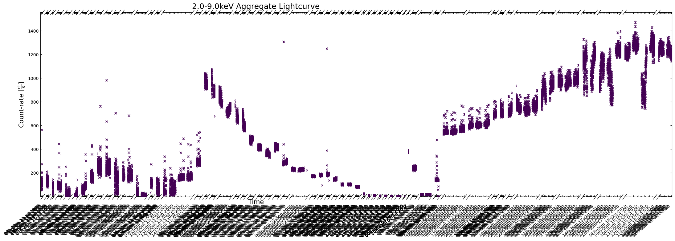
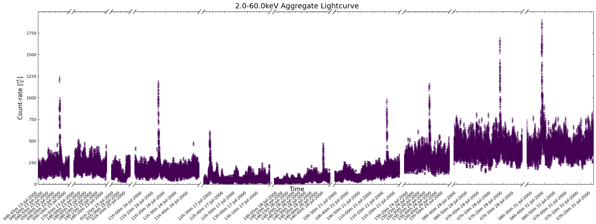
Examining long-term variability#
As we noted earlier, the RXTE observations that we selected were taken over the course of more than 10 years, and as such we have the opportunity to explore how the X-ray emission of T5X2 has altered in the long term (long term to a human anyway).
This is another reason that we chose to read in our archived light curves as XGA LightCurve objects; they make it easy to manage a large collection of light curves taken over a long period of time, organize them, and then extract some insights.
A list of XGA LightCurve objects can be used to set up another type of XGA
product, an AggregateLightCurve, which handles the management of a large, unwieldy
set of light curves. It will ensure that the light curves are sorted by time, will check
that they have consistent energy bands and time bins, and also provide a simple
way to access the data of all the constituent light curves together.
The AggregateLightCurve class also includes convenient visualization functions.
If the archived RXTE-PCA and HEXTE light curves had the same time bin size and energy
bands, we would be able to put them all into a single AggregateLightCurve, providing
convenient access to the data of all the light curves at once. We would also be able to
include light curves from other telescopes, which would also be sorted and made easily
accessible by the AggregateLightCurve object.
However, as the time bin sizes and energy bands are not consistent between these
instruments, we’ll have to set up a few different AggregateLightCurve objects:
# Very ugly definition of a nested dictionary of AggregateLightCurve objects
agg_lcs = {
    "PCA": {
        "{0}-{1}keV".format(*e.value): AggregateLightCurve(
            like_lcs["PCA"]["{0}-{1}keV".format(*e.value)]
        )
        for e in PCA_EN_BANDS.values()
    },
    "HEXTE": {
        "{0}-{1}keV".format(*e.value): AggregateLightCurve(
            like_lcs["HEXTE-0"]["{0}-{1}keV".format(*e.value)]
            + like_lcs["HEXTE-1"]["{0}-{1}keV".format(*e.value)]
        )
        for e in HEXTE_EN_BANDS.values()
    },
}

agg_lcs
{'PCA': {'2.0-9.0keV': <xga.products.lightcurve.AggregateLightCurve at 0x7f33a1241340>,
  '2.0-4.0keV': <xga.products.lightcurve.AggregateLightCurve at 0x7f33a107b9b0>,
  '4.0-9.0keV': <xga.products.lightcurve.AggregateLightCurve at 0x7f33a0eab5f0>,
  '9.0-20.0keV': <xga.products.lightcurve.AggregateLightCurve at 0x7f33a3e7e480>,
  '20.0-40.0keV': <xga.products.lightcurve.AggregateLightCurve at 0x7f33a0d27d40>},
 'HEXTE': {'15.0-30.0keV': <xga.products.lightcurve.AggregateLightCurve at 0x7f33a3e8e270>,
  '30.0-60.0keV': <xga.products.lightcurve.AggregateLightCurve at 0x7f33a0d27740>,
  '60.0-250.0keV': <xga.products.lightcurve.AggregateLightCurve at 0x7f33a0acddf0>}}
Interacting with aggregate light curves#
What you want to do with your aggregated light curve and the long-term variability that it describes (depending on what your source is and how many times it was observed, of course) will depend heavily on your particular science case.
We will now demonstrate how to access and interact with the data, using the 2–9 keV PCA aggregate light curve as an example.
demo_agg_lc = agg_lcs["PCA"]["2.0-9.0keV"]
demo_agg_lc
<xga.products.lightcurve.AggregateLightCurve at 0x7f33a1241340>
Which observations contributed data?#
As AggregateLightCurves are particularly well suited for providing an interface to
the time variability of a source that has been observed many times, such as T5X2, we
might conceivably lose track of which observations (denoted by their ObsID)
contributed data.
In this demonstration, for instance, we just identified the relevant observations and downloaded them, without closely examining which ObsIDs we were actually using.
The obs_ids property will return a dictionary that stores the relevant ObsIDs, with
the dictionary keys being the names of the telescopes from which the data were taken:
pprint(demo_agg_lc.obs_ids, compact=True)
{'RXTE': ['50138030100', '50138030101', '50138030200', '50138030300',
          '50138030400', '50138030500', '50054060100', '50054060101',
          '50054060200', '50054060201', '50054060202', '50054060300',
          '50054060301', '50054060401', '50054060402', '50054060400',
          '50054060403', '50054060500', '50054060501', '50054060600',
          '50054060601', '50054060700', '50054060701', '50054060802',
          '50054060900', '50054060901', '50054061000', '50054061001',
          '50054061100', '50054061101', '50054061102', '50054061200',
          '50054061201', '50054061203', '50054061202', '50054061300',
          '50054061301', '50054061400', '50054061401', '50054061500',
          '50054061501', '50054061502', '50054061503', '70412010100',
          '70412010200', '70412010300', '95437010100', '95437010200',
          '95437010201', '95437010300', '95437010301', '95437010302',
          '95437010303', '95437010400', '95437010401', '95437010500',
          '95437010501', '954370106000', '95437010600']}
Both the telescope names and the instruments associated with each ObsID are accessible through their own properties:
demo_agg_lc.telescopes
['RXTE']
pprint(demo_agg_lc.instruments, compact=True)
{'RXTE': {'50054060100': ['PCA'],
          '50054060101': ['PCA'],
          '50054060200': ['PCA'],
          '50054060201': ['PCA'],
          '50054060202': ['PCA'],
          '50054060300': ['PCA'],
          '50054060301': ['PCA'],
          '50054060400': ['PCA'],
          '50054060401': ['PCA'],
          '50054060402': ['PCA'],
          '50054060403': ['PCA'],
          '50054060500': ['PCA'],
          '50054060501': ['PCA'],
          '50054060600': ['PCA'],
          '50054060601': ['PCA'],
          '50054060700': ['PCA'],
          '50054060701': ['PCA'],
          '50054060802': ['PCA'],
          '50054060900': ['PCA'],
          '50054060901': ['PCA'],
          '50054061000': ['PCA'],
          '50054061001': ['PCA'],
          '50054061100': ['PCA'],
          '50054061101': ['PCA'],
          '50054061102': ['PCA'],
          '50054061200': ['PCA'],
          '50054061201': ['PCA'],
          '50054061202': ['PCA'],
          '50054061203': ['PCA'],
          '50054061300': ['PCA'],
          '50054061301': ['PCA'],
          '50054061400': ['PCA'],
          '50054061401': ['PCA'],
          '50054061500': ['PCA'],
          '50054061501': ['PCA'],
          '50054061502': ['PCA'],
          '50054061503': ['PCA'],
          '50138030100': ['PCA'],
          '50138030101': ['PCA'],
          '50138030200': ['PCA'],
          '50138030300': ['PCA'],
          '50138030400': ['PCA'],
          '50138030500': ['PCA'],
          '70412010100': ['PCA'],
          '70412010200': ['PCA'],
          '70412010300': ['PCA'],
          '95437010100': ['PCA'],
          '95437010200': ['PCA'],
          '95437010201': ['PCA'],
          '95437010300': ['PCA'],
          '95437010301': ['PCA'],
          '95437010302': ['PCA'],
          '95437010303': ['PCA'],
          '95437010400': ['PCA'],
          '95437010401': ['PCA'],
          '95437010500': ['PCA'],
          '95437010501': ['PCA'],
          '95437010600': ['PCA'],
          '954370106000': ['PCA']}}
demo_agg_lc.associated_instruments
{'RXTE': ['PCA']}
Retrieving constituent light curves#
Though the AggregateLightCurve object provides a convenient way to access the data of all the light curves that it contains, you might sometimes want to retrieve the individual LightCurve objects.
Using the get_lightcurves() method, you can retrieve LightCurve objects for
particular time chunks:
demo_agg_lc.get_lightcurves(0)
<xga.products.lightcurve.LightCurve at 0x7f33a0ea9070>
If the AggregateLightCurve contains data from multiple instruments, telescopes, or
ObsIDs, then the inst, telescope, and obs_id arguments can be passed.
Accessing all data#
demo_agg_lc.get_data()
(<Quantity [  94.79163,   72.70727,   96.5273 , ..., 1238.7705 , 1230.9957 ,
            1212.9932 ] ct / s>,
 <Quantity [2.505628, 2.216513, 2.526862, ..., 8.773673, 8.746537, 8.682692] ct / s>,
 array([2.06081059e+08, 2.06081075e+08, 2.06081091e+08, ...,
        5.30035603e+08, 5.30035619e+08, 5.30035635e+08], shape=(13915,)),
 array([ 0,  0,  0, ..., 58, 58, 58], shape=(13915,)))
Accessing data for a specific time interval#
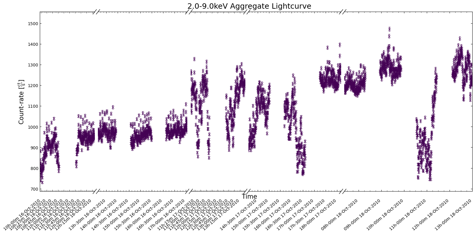
This part of the demonstration will show you how to access data within specific time intervals of interest - we define the following start and stop times based on an interesting time window discussed in M. Linares et al. (2012):
demo_agg_wind_start = Time("2010-10-16 09:00:00")
demo_agg_wind_stop = Time("2010-10-18 12:00:00")
An AggregateLightCurve’s constituent products are organized into discrete ‘time chunks’, defined by a start and stop time that do not overlap with any other ‘time chunk’. Time chunks are sorted so that their ‘time chunk ID’, which uniquely identifies them, represents where they are in the sorted list of time chunks (i.e., time chunk 1 contains data taken after time chunk 0, and so on).
Looking at the time_chunk_ids property shows us how many time chunks this
set of PCA light curves is divided into:
demo_agg_lc.time_chunk_ids
array([ 0,  1,  2,  3,  4,  5,  6,  7,  8,  9, 10, 11, 12, 13, 14, 15, 16,
       17, 18, 19, 20, 21, 22, 23, 24, 25, 26, 27, 28, 29, 30, 31, 32, 33,
       34, 35, 36, 37, 38, 39, 40, 41, 42, 43, 44, 45, 46, 47, 48, 49, 50,
       51, 52, 53, 54, 55, 56, 57, 58])
The time intervals represented by those IDs are also accessible, with the first column
containing the start time of the time chunk, and the second column containing the
stop time. This information is available both in the form of seconds
from the reference time (time_chunks), and the other in the form of explicit
datetime objects (datetime_chunks):
demo_agg_lc.time_chunks[:10]
demo_agg_lc.datetime_chunks[:10]
array([[datetime.datetime(2000, 7, 13, 4, 45, 15, 562431),
        datetime.datetime(2000, 7, 13, 5, 12, 11, 562431)],
       [datetime.datetime(2000, 7, 13, 17, 53, 31, 562431),
        datetime.datetime(2000, 7, 13, 18, 22, 3, 562431)],
       [datetime.datetime(2000, 7, 15, 1, 23, 39, 562431),
        datetime.datetime(2000, 7, 15, 1, 38, 51, 562431)],
       [datetime.datetime(2000, 7, 16, 10, 52, 59, 562431),
        datetime.datetime(2000, 7, 16, 11, 47, 23, 562431)],
       [datetime.datetime(2000, 7, 17, 12, 23, 23, 562431),
        datetime.datetime(2000, 7, 17, 13, 18, 3, 562431)],
       [datetime.datetime(2000, 7, 18, 14, 0, 27, 562431),
        datetime.datetime(2000, 7, 18, 14, 48, 27, 562431)],
       [datetime.datetime(2000, 7, 21, 10, 26, 51, 562431),
        datetime.datetime(2000, 7, 21, 11, 21, 47, 562431)],
       [datetime.datetime(2000, 7, 24, 15, 15, 39, 562431),
        datetime.datetime(2000, 7, 24, 15, 53, 31, 562431)],
       [datetime.datetime(2000, 7, 28, 6, 38, 51, 562431),
        datetime.datetime(2000, 7, 28, 7, 34, 51, 562431)],
       [datetime.datetime(2000, 7, 31, 6, 23, 23, 562431),
        datetime.datetime(2000, 7, 31, 7, 20, 27, 562431)]], dtype=object)
We can use the obs_ids_within_interval() method to identify which observations
took place within a given time interval:
demo_agg_lc.obs_ids_within_interval(demo_agg_wind_start, demo_agg_wind_stop)
{'RXTE': ['95437010400',
  '95437010401',
  '95437010500',
  '95437010501',
  '954370106000']}
The default behavior of this method is to
return ObsIDs of observations that overlap with the interval, but if you
pass over_run=False then only ObsIDs of observations that took place entirely within
the specified interval will be returned:
demo_agg_lc.obs_ids_within_interval(
    demo_agg_wind_start, demo_agg_wind_stop, over_run=False
)
{'RXTE': ['95437010400', '95437010401', '95437010500', '95437010501']}
That method makes use of the time_chunk_ids_within_interval() method, which you can
use in exactly the same way to retrieve the time chunk IDs that are part of a given
time interval:
demo_agg_lc.time_chunk_ids_within_interval(demo_agg_wind_start, demo_agg_wind_stop)
array([53, 54, 55, 56, 57])
Visualizing aggregated light curves#
We can use the view() method to quickly produce a plot of the aggregated light curve, but if your
dataset covers a particularly long time period, you can end up with a very unhelpful figure:
demo_agg_lc.view(show_legend=False)
To address the problems with the last figure, we could increase its size by passing a custom value to
the figsize argument (e.g. (30, 6)), or you could specify a particular time window to focus on:
demo_agg_lc.view(
    interval_start=demo_agg_wind_start,
    interval_end=demo_agg_wind_stop,
    show_legend=False,
)
4. Generating new RXTE-PCA light curves#
The time bin size of archived RXTE light curves is relatively coarse, particularly compared to the time resolution that the PCA and HEXTE instruments can achieve. Given the type of object we are investigating, we might reasonably expect that significant emission variations might be happening at smaller time scales than our time bin size.
Our inspiration for this demonstration, the work by M. Linares et al. (2012), generated RXTE-PCA light curves with different time bin sizes (2-second and 1-second bins) to search for different features.
Also, while light curves generated within several different energy bands are included in the RXTE archive, many science cases will require that light curves be generated in very specific energy bands.
The archived light curves have gotten our exploration of T5X2’s variable X-ray emission off to an excellent start, but clearly we also need to be able to generate new versions that are tailored to our specific requirements.
This section of the notebook will go through the steps required to make RXTE-PCA light curves from scratch, focusing on the two requirements mentioned above; smaller time bins, and control over light curve energy bands.
Downloading specific files for our RXTE observations#
Unfortunately, our first step is to spend even more time downloading data from the RXTE archive, as we previously targeted only the archived light curve files. Making new light curves requires all the original data and many spacecraft files.
The RXTE archive does not contain equivalents of the pre-cleaned event files found in many other HEASARC-hosted high-energy telescope archives, which is why we will have to perform the calibration and reduction processes from scratch.
We could use the Astroquery Heasarc.download_data() object to download whole directories for all observations, just as
we demonstrated in the first part of Section 2, e.g.:
Heasarc.download_data(data_links, host="aws", location=ROOT_DATA_DIR)
However, to save some downloading time and storage space, we will take a slightly more complex approach and download only the files we’re going to need to reprocess the observations and generate new light curves.
We defined a list of files and directories that we do not need to download (DOWN_EXCLUDE) in the
‘Global Setup: Constants’ section near the top of the notebook, and we will use it in combination with
the s3fs Python module to list and filter the files in each observation’s directory.
Then we will use s3fs to download just those files that we need:
for dl in data_links:
    cur_uri = dl["aws"]
    all_cont = np.array(
        s3.ls(
            cur_uri,
        )
    )
    down_mask = np.all(np.char.find(all_cont, DOWN_EXCLUDE[..., None]).T == -1, axis=1)
    down_cont = all_cont[down_mask].tolist()

    infer_oi = os.path.dirname(cur_uri).split("/")[-1]

    cur_out = os.path.join(ROOT_DATA_DIR, infer_oi)
    os.makedirs(cur_out, exist_ok=True)

    for cur_down_cont in down_cont:
        s3.get(cur_down_cont, cur_out, recursive=True, on_error="ignore")
Note
We note that it is generally recommended to reprocess high-energy event lists taken from HEASARC mission archives from scratch, as it means that the latest calibration and filtering procedures can be applied.
Running the RXTE-PCA preparation pipeline#
A convenient pipeline to prepare RXTE-PCA data for use is included in the HEASoft
package - pcaprepobsid. It will take us from raw RXTE-PCA data to the science-ready
data and filter files required to generate light curves in a later step - the PCA team
recommended the default configuration of the pipeline for general scientific use.
Now we have to talk about the slightly unusual nature of RXTE-PCA observations; the PCA proportional counter units could be simultaneously read out in various ‘data modes’. That meant that some limitations of the detectors and electronics could be mitigated by using data from the different modes in different parts of your analysis.
At least 10 different data modes could be requested by the observer, but the ‘Standard-1’ and ‘Standard-2’ modes were active for every observation.
The RXTE-PCA instrument had very high temporal and moderate spectral resolutions, but both could not be true at the same time. The ‘Standard-1’ and ‘Standard-2’ modes ‘binned’ the readout from the detectors in two different ways:
Standard 1 - accumulated the combined readout from all detector channels, with a time resolution of 0.125 seconds.
Standard 2 - accumulated the 256 detector channels binned into 129 ‘Standard 2’ channels, with a time resolution of 16 seconds.
Note
The Standard-2 data mode is the most commonly used and supported.
We are using the HEASoftPy interface to the pcaprepobsid task, but wrap it in
another function (defined in the ‘Global Setup’ section) that makes it easier for us
to run the processing of different observation’s PCA data in parallel.
As the initial processing of raw data is the step in any analysis most likely to error, we have made sure that the wrapper function returns information on whether the processing failed, the logs, and the relevant ObsID. That makes it easy for us to identify problem ObsIDs.
Now we run the pipeline for all of our selected RXTE observations:
with mp.Pool(NUM_CORES) as p:
    arg_combs = [[oi, os.path.join(OUT_PATH, oi), rel_coord] for oi in rel_obsids]
    pipe_result = p.starmap(process_rxte_pca, arg_combs)

pca_pipe_problem_ois = [
    all_out[0]
    for all_out in pipe_result
    if not all_out[2]
    or "Task pcaprepobsid 1.4 terminating with status -1" in str(all_out[1])
]
rel_obsids = [oi for oi in rel_obsids if oi not in pca_pipe_problem_ois]

pca_pipe_problem_ois
/opt/envs/heasoft/lib/python3.12/multiprocessing/popen_fork.py:66: DeprecationWarning: This process (pid=2039) is multi-threaded, use of fork() may lead to deadlocks in the child.
  self.pid = os.fork()
['50054-06-08-00', '50054-06-08-01', '50054-06-08-03', '50054-06-08-04']
Setting up RXTE-PCA good time interval (GTI) files#
The RXTE-PCA data for our observations of T5X2 are now (sort of) ready for use!
Though the observation data files have been prepared, we do still need to define
‘good time interval’ (GTI) files for each observation. These will combine the filter
file produced by pcaprepobsid, which is determined by various spacecraft orbit and
electronics housekeeping considerations, with another user-defined filtering expression.
The user-defined filter is highly customizable, but we will use the expression recommended (see the note below for the source of this recommendation) to apply ‘basic’ screening to RXTE-PCA observations of a bright target:
# Recommended filtering expression from RXTE cookbook pages
filt_expr = "(ELV > 4) .AND. (OFFSET < 0.1) .AND. (NUM_PCU_ON > 0 .AND. NUM_PCU_ON < 6)"
Breaking down the terms of the filter expression:
ELV > 4 - Ensures that the target is above the Earth’s horizon. More conservative limits (e.g., > 10) will make sure that ‘bright earth’ is fully screened out, but this value is sufficient for many cases.
OFFSET < 0.1 - Makes sure that PCA is pointed at the target to within 0.1 degrees.
NUM_PCU_ON > 0 .AND. NUM_PCU_ON < 6 - Ensures that at least one of the five proportional counter units is active.
See also
An in-depth discussion of how to screen/filter RXTE-PCA data is available on the HEASARC website.
Now that we’ve settled on the filtering expression, the maketime HEASoft task can
be used to make the final GTI files for each observation. Another wrapper function to
the HEASoftPy maketime interface is declared, and we again execute the task in parallel:
with mp.Pool(NUM_CORES) as p:
    arg_combs = [[oi, os.path.join(OUT_PATH, oi), filt_expr] for oi in rel_obsids]
    gti_result = p.starmap(gen_pca_gti, arg_combs)
New light curves within custom energy bounds#
Recall that we want to generate two categories of custom light curves; those within custom energy bands, and those with time resolution better than 16 seconds.
We’ll tackle the custom energy band light curves first, as they use the more common
data mode, ‘Standard-2’. The generation of these light curves will be
straightforward, as HEASoft includes a task called pcaextlc2 for exactly this
purpose.
As previously mentioned, the RXTE-PCA instrument is made up of five separate proportional counter units (PCUs). The state and reliability of those PCUs varied significantly over the lifetime of the mission, so we do not necessarily use want to use data from all five.
PCU 2 was considered the most reliable, and so we are going to use that for our newly generated light curves.
chos_pcu_id = "2"
Note
The default behaviour of PCA light curve generation functions in HEASoft is to use all available PCUs, in which case a combined light curve is produced. We have set up our wrapper functions for the light curve generation tasks so that a single PCU or a list of PCUs can be passed.
The slight sticking point is that pcaextlc2 takes arguments of upper and
lower absolute channel limits to specify which band the output light curve should be
generated within. Our particular science case will inform us which energy bands
we should look at, but we have to convert them to channels ourselves.
Caution
It is important to make a distinction between RXTE-PCA ‘Standard-2’ channels (which have values between 0 and 128) and PCA’s absolute channels (which have values between 0 and 255). Standard-2 is a binned data mode, and its channels represent combinations of absolute channels.
We need to convert our energy bands (whatever we decide they will be) to the equivalent absolute channels. HEASARC provides a table that describes the mapping of absolute channels to ‘Standard-2’ channels and energies at different epochs in the life of the telescope.
You could quite easily use this to convert from your target energy band to the absolute channel limits, but when dealing with many archival observations from different epochs, it is more convenient to implement a more automated solution.
Building RXTE-PCA response files#
That automated method of converting from energy to channel involves:
Generating new RXTE-PCA response files for each observation
Using the “EBOUNDS” table of responses to move from energy to ‘Standard-2’ channel
Finally, using the known binning of ‘Standard-2’ channels to arrive at the absolute channel limits.
We note that as some, but not all, ‘Standard-2’ channels correspond to a range of absolute channels, the mean value of the absolute channel range is used, and rounded down to the nearest integer for the lower limit, and rounded up to the nearest integer for the upper limit.
Rather than using the HEASoft tool specifically for generating RXTE-PCA RMFs, we
cheat a little and use the HEASoft tool designed to produce spectra (and supporting
files) from RXTE-PCA data; pcaextspect2.
The advantage of this is that pcaextspect2 will automatically handle the combination
of responses from different PCUs, which would not be necessary for our use of PCU 2, but
makes it easier to use multiple PCUs if you choose.
As with the other HEASoft tasks, we write a wrapper function for the HEASoftPy interface in order to run the task in parallel:
with mp.Pool(NUM_CORES) as p:
    arg_combs = [[oi, os.path.join(OUT_PATH, oi), chos_pcu_id] for oi in rel_obsids]
    rsp_result = p.starmap(gen_pca_s2_spec_resp, arg_combs)
Note
The response files produced by pcaextspect2 are a combination of the ARF and RMF
products commonly seen in high energy astrophysics data.
To make the next step easier, we set up a template for the path to the response files we just generated:
rsp_path_temp = os.path.join(OUT_PATH, "{oi}", "rxte-pca-pcu{sp}-{oi}.rsp")
Generating the light curves#
Now that the response files have been generated, we can create our new light curves!
The first step is to decide on the lower and upper limits of the energy band(s) we want the light curve(s) to be drawn from. We also define the time bin size to use, remembering that the ‘Standard-2’ data mode required for applying energy bounds has a minimum time resolution of 16 seconds.
We choose to build light curves in three custom energy bands:
2-10 keV
10-30 keV
2-60 keV
These selections are fairly arbitrary and aren’t physically justified, but yours
should be informed by your science case. If you are using this code as a template
for your own analysis, you could add more energy bands to the new_lc_en_bnds list,
and they would be generated as well.
We choose a time bin size of 16 seconds, as this is a bright source and we wish for the best possible temporal resolution.
new_lc_en_bnds = [
    Quantity([2, 10], "keV"),
    Quantity([10, 30], "keV"),
    Quantity([2, 60], "keV"),
]

en_time_bin_size = Quantity(16, "s")
Now we can run the pcaextlc2 task to generate the light curves. We note that the
wrapper function we create for the HEASoftPy interface to pcaextlc2 includes
extra processing steps that use the supplied lower and upper energy limits and
response file to determine the absolute channel limits. Please examine the
wrapper function defined in the ‘Global Setup’ section for more details.
form_sel_pcu = pca_pcu_check(chos_pcu_id)

with mp.Pool(NUM_CORES) as p:
    arg_combs = [
        [
            oi,
            os.path.join(OUT_PATH, oi),
            *cur_bnds,
            rsp_path_temp.format(oi=oi, sp=form_sel_pcu),
            en_time_bin_size,
            chos_pcu_id,
        ]
        for oi in rel_obsids
        for cur_bnds in new_lc_en_bnds
    ]
    lc_en_result = p.starmap(gen_pca_s2_light_curve, arg_combs)
Finally, we set up a template for the path to the light curves we just generated:
lc_path_temp = os.path.join(
    OUT_PATH, "{oi}", "rxte-pca-pcu{sp}-{oi}-en{lo}_{hi}keV-tb{tb}s-lightcurve.fits"
)
Loading the light curves into Python#
Our shiny new custom-energy-band light curves can be loaded into convenient XGA LightCurve objects, just as the archived light curves were - they will once again provide a convenient interface to the data, and some nice visualization capabilities.
As we set up the energy bands in which to generate new light curves as a list of Astropy quantities (which you may add to or remove from for your own purposes), and we know the format of the output file names (as we set that up), we can dynamically load in those light curves.
Iterating through the energy bounds, and the relevant ObsIDs, every new light curve file gets its own LightCurve object, and is then appended to a list in a dictionary with energy bands as keys.
From there, one aggregate light curve per energy band is set up and also stored in a dictionary for easy (and dynamic) access:
gen_en_bnd_lcs = {}

for cur_bnd in new_lc_en_bnds:
    cur_bnd_key = "{0}-{1}keV".format(*cur_bnd.value)
    gen_en_bnd_lcs.setdefault(cur_bnd_key, [])

    for oi in rel_obsids:
        cur_lc_path = lc_path_temp.format(
            oi=oi,
            sp=form_sel_pcu,
            tb=en_time_bin_size.value,
            lo=cur_bnd[0].value,
            hi=cur_bnd[1].value,
        )

        cur_lc = LightCurve(
            cur_lc_path,
            oi,
            "PCA",
            "",
            "",
            "",
            rel_coord_quan,
            Quantity(0, "arcmin"),
            RXTE_AP_SIZES["PCA"],
            *cur_bnd,
            en_time_bin_size,
            telescope="RXTE",
        )

        gen_en_bnd_lcs[cur_bnd_key].append(cur_lc)

# Set up the aggregate light curves
agg_gen_en_bnd_lcs = {
    cur_bnd_key: AggregateLightCurve(cur_bnd_lcs)
    for cur_bnd_key, cur_bnd_lcs in gen_en_bnd_lcs.items()
}

# Show the structure of the agg_gen_en_bnd_lcs dictionary
agg_gen_en_bnd_lcs
{'2.0-10.0keV': <xga.products.lightcurve.AggregateLightCurve at 0x7f337b43fb30>,
 '10.0-30.0keV': <xga.products.lightcurve.AggregateLightCurve at 0x7f337b5538f0>,
 '2.0-60.0keV': <xga.products.lightcurve.AggregateLightCurve at 0x7f337bd0ea20>}
Visualizing new custom-energy-band light curves#
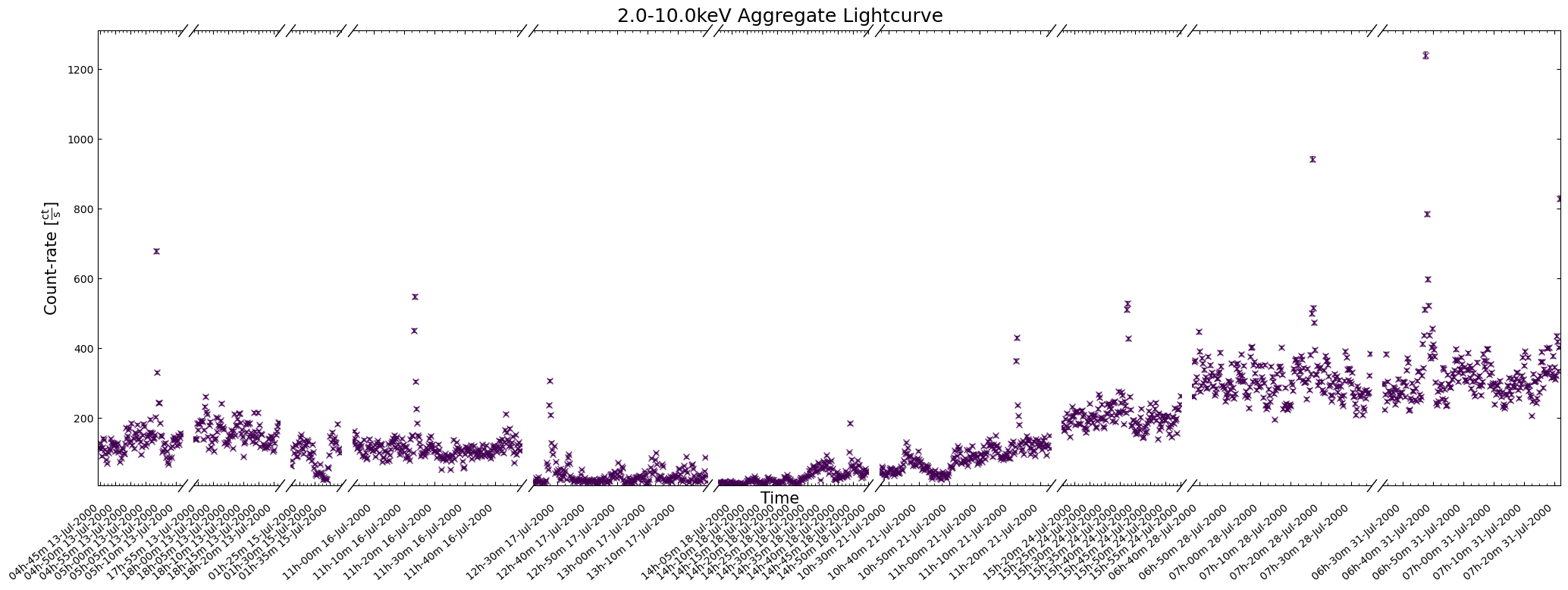
The first thing to do is to take a look at one of our new light curves to make sure that (on the surface at least) everything looks reasonably sensible.
You should really examine the whole aggregation of new light curves in a particular energy band, but for demonstrative purposes we’ll look at a two-week time window:
agg_gen_en_bnd_lcs["2.0-10.0keV"].view(
    show_legend=False,
    figsize=(18, 6),
    interval_start=Time("2000-07-13 05:00:00"),
    interval_end=Time("2000-08-03"),
)
Calculating and examining hardness ratio curves#
Being able to generate light curves within energy bands of our choice will be a useful tool for many science cases; for instance, sometimes you wish to target particular emission mechanisms that produce X-ray photons of a certain energy.
Sometimes you take a broader view and simply want to know if the variation in emission is distinct between the ‘soft’ X-ray band to the ‘hard’ X-ray band (exactly what defines ‘hard’ and ‘soft’ will vary depending on your specialization, the telescope you’re using, and sometimes just how you feel on a particular day).
In either case it is often useful to visualize a ‘hardness curve’ which shows how the ‘hardness ratio’ of two energy bands changes with time. There are multiple definitions of the hardness ratio, but for our purposes we’ll use:
Where \(\rm{HR}_{{H:S}}\) is the hard-to-soft band ratio, \(F_{H}\) is the flux in the hard band, and \(F_{S}\) is the flux in the soft band.
Hardness curves can be considered as a short-cut to the sort of information extracted from time-resolved spectroscopy (which is outside the scope of this tutorial).
See also
Our calculation of hardness ratio is fairly simplistic - there are better approaches that take into account the often-Poissian nature of X-ray light curve data points, and calculate uncertainties on the ratio. See the Chandra Source Catalog hardness ratio page for an example.
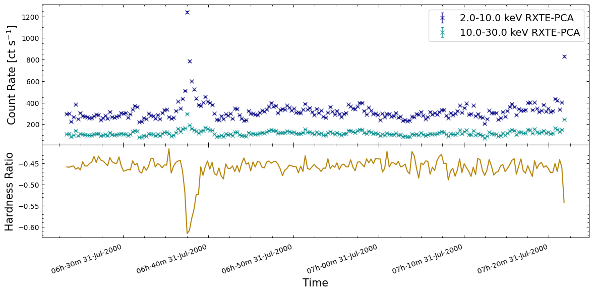
We will choose a single observation to visualize the hardness ratio curve for, just for ease of viewing; there is no reason you could not use the same approach for all observations.
Three energy-bands were chosen when we generated the new light curves earlier in this section, and we will choose the 2.0–10 keV as the soft band, and the 10.0–30 keV as the hard band:
hard_rat_ch_id = 9

lo_en_demo_lc = agg_gen_en_bnd_lcs["2.0-10.0keV"].get_lightcurves(hard_rat_ch_id)
hi_en_demo_lc = agg_gen_en_bnd_lcs["10.0-30.0keV"].get_lightcurves(hard_rat_ch_id)

hard_rat = (hi_en_demo_lc.count_rate - lo_en_demo_lc.count_rate) / (
    hi_en_demo_lc.count_rate + lo_en_demo_lc.count_rate
)
The figure we produce plots the two light curves on the same axis, and then the calculated hardness curve on a second axis below. As such, we can both see the original behaviors evident in the light curves, and how the hardness ratio changes for those behaviors.
We find that the hardness ratio is effectively constant for much of the chosen observation, and that the approximately constant value indicates that more emission is detected in the soft band than the hard.
Interestingly, when we see a very large increase in emission from a burst, the hardness ratio drops significantly, becoming even more negative. Thinking back to the hardness ratio definition, it is clear that these large bursts emit more photons in the soft-band (2–10 keV in this case) than the hard-band (10–30 keV).
Interpreting this sort of behavior is heavily dependent on your science case and the astrophysics involved in whatever object you are studying. However, our initial hypothesis here might be that the large bursts originate from a different mechanism than the smaller variations in emission we see elsewhere in the light curves.
New light curves with high temporal resolution#
Addressing our other reason for generating new light curves, we can now use the ‘Standard-1’ data mode to achieve a much finer temporal resolution than the ‘Standard-2’ mode.
We select a time bin size of 2 seconds to match the temporal resolution of the RXTE-PCA light curves that M. Linares et al. (2012) used to identify T5X2 bursts:
new_lc_time_bin_sizes = Quantity([1, 2], "s")
This is still considerably oversampling the potential time resolution for ‘Standard-1’ data, as it is binned into 0.125 second chunks.
Generating new light curves#
Unlike when we made new light curves within a custom energy band, we don’t need to worry about converting from energy to channels as, unfortunately, ‘Standard-1’ data does not contain any spectral information.
Warning
Though ‘Standard-1’ data contains no spectral information (as it consists of the
combined readout from all detector channels) the pcaextlc1 HEASoft task does
take minimum and maximum channel arguments - do not use them.
Here we wrap and run the pcaextlc1 task in parallel, just as we did pcaextlc2 in the last section:
form_sel_pcu = pca_pcu_check(chos_pcu_id)

with mp.Pool(NUM_CORES) as p:
    arg_combs = [
        [
            oi,
            os.path.join(OUT_PATH, oi),
            cur_tsz,
            chos_pcu_id,
        ]
        for oi in rel_obsids
        for cur_tsz in new_lc_time_bin_sizes
    ]
    lc_result = p.starmap(gen_pca_s1_light_curve, arg_combs)
/opt/envs/heasoft/lib/python3.12/multiprocessing/popen_fork.py:66: DeprecationWarning: This process (pid=2039) is multi-threaded, use of fork() may lead to deadlocks in the child.
  self.pid = os.fork()
Finally, we set up a template for the path to the light curves we just generated:
lc_hi_res_path_temp = os.path.join(
    OUT_PATH, "{oi}", "rxte-pca-pcu{sp}-{oi}-enALL-tb{tb}s-lightcurve.fits"
)
Loading the light curves into Python#
Just as we did for the archived light curves and the newly generated energy-bound light curves, we will load the new files into XGA LightCurve objects, and from there into an AggregateLightCurve per time-bin-size:
gen_hi_time_res_lcs = {}

for cur_tsz in new_lc_time_bin_sizes:
    cur_tsz_key = cur_tsz.to_string().replace(" ", "")
    gen_hi_time_res_lcs.setdefault(cur_tsz_key, [])

    for oi in rel_obsids:
        cur_lc_path = lc_hi_res_path_temp.format(
            oi=oi, sp=form_sel_pcu, tb=cur_tsz.value
        )

        cur_lc = LightCurve(
            cur_lc_path,
            oi,
            "PCA",
            "",
            "",
            "",
            rel_coord_quan,
            Quantity(0, "arcmin"),
            RXTE_AP_SIZES["PCA"],
            Quantity(2, "keV"),
            Quantity(60, "keV"),
            cur_tsz,
            telescope="RXTE",
        )

        gen_hi_time_res_lcs[cur_tsz_key].append(cur_lc)

# Set up the aggregate light curves
agg_gen_hi_time_res_lcs = {
    cur_tsz_key: AggregateLightCurve(cur_tsz_lcs)
    for cur_tsz_key, cur_tsz_lcs in gen_hi_time_res_lcs.items()
}

# Show the structure of the agg_gen_hi_time_res_lcs dictionary
agg_gen_hi_time_res_lcs
{'1.0s': <xga.products.lightcurve.AggregateLightCurve at 0x7f33cce366c0>,
 '2.0s': <xga.products.lightcurve.AggregateLightCurve at 0x7f33ccd89340>}
Visualizing new higher time-resolution light curves#
We can now visually examine the new higher-temporal-resolution light curves. It is always good practice to visually examine your data, as it can help you spot any potential problems, as well as any interesting features.
There are new light curves with both one-second and two-second time bins, but here we will select the highest-resolution option to examine.
Rather than looking at the whole aggregate light curve, we choose a small date range to increase the interpretability of the output figure:
To give a sense of how the finer temporal bins might affect our interpretation of our source’s (T5X2) time-varying behavior, we are going to plot a single observation’s light curve generated with one, two, and sixteen second time bins.
The sixteen-second time bin light curve is in the same energy band as the two fine-temporal-resolution light curves (2–60 keV), and was generated in the “New light curves within custom energy bounds” section of this notebook.
We access the relevant aggregate light curves and extract a single light curve from each - the selected light curves are all from the same time bin (thus observation), as we wish to compare like-to-like:
tbin_comp_ch_id = 9

onesec_demo_lc = agg_gen_hi_time_res_lcs["1.0s"].get_lightcurves(tbin_comp_ch_id)
twosec_demo_lc = agg_gen_hi_time_res_lcs["2.0s"].get_lightcurves(tbin_comp_ch_id)

sixteensec_demo_lc = agg_gen_en_bnd_lcs["2.0-60.0keV"].get_lightcurves(tbin_comp_ch_id)
Plotting the light curves on the same axis is an excellent demonstration of why we bothered to make new light curves with finer time binning in the first place.
The default sixteen-second binning clearly obfuscates many of the smaller, shorter timescale, variations in T5X2’s 2–60 keV X-ray emission. Larger features are still clear, though broadened by the coarser time bins, but finer time bins reveal a lot of interesting features:
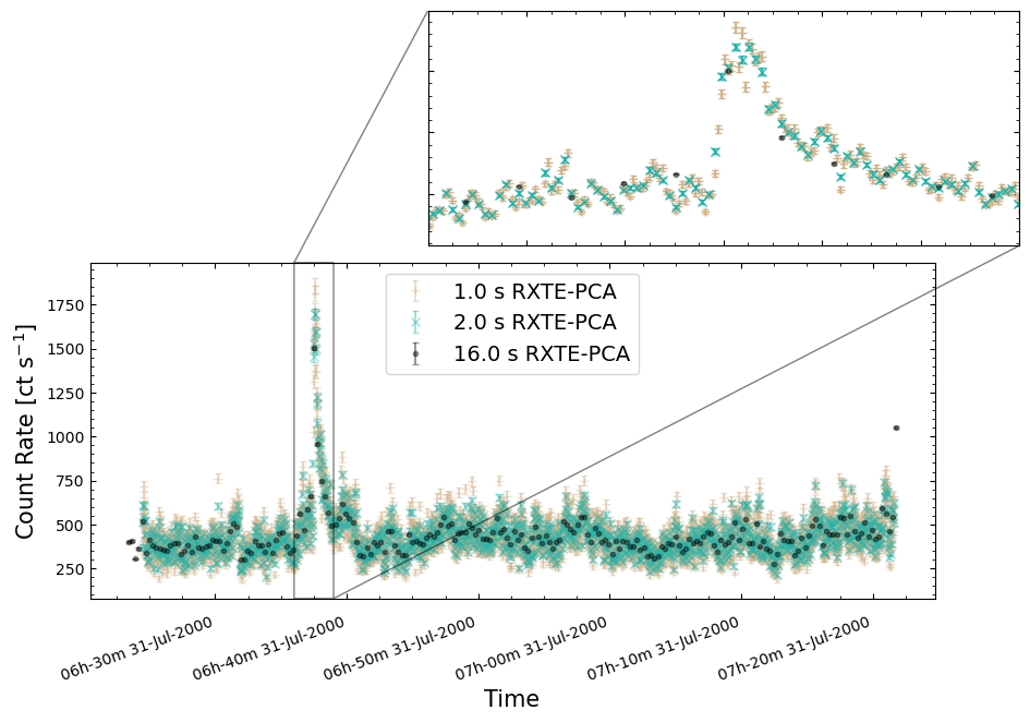
5. Experimenting with an automated method to identify bursts#
For the final step of this demonstration, we will experiment with automated ways to identify when T5X2 bursts occur. The work by M. Linares et al. (2012) that inspired this tutorial identified bursts by manual inspection of light curves with two-second time resolution.
Manual inspection by experts is often the most reliable way to identify features like bursts, even though it is possible it may introduce unquantifiable human error and biases.
Such manual inspection is unfortunately very time-consuming, and factors such as decision fatigue (see M. Maier et al. 2024, for a review of decision fatigue in medical decision-making) can cause a variation in the inspector’s performance over the course of the task.
As such, and because it is an interesting thing to do with the light curves we have just generated, we will attempt the same task algorithmically.
We match the light curves used for burst identification by M. Linares et al. (2012), choosing our new two-second time bin light curves to experiment with. An individual light curve from that aggregated light curve is also selected for testing purposes:
burst_id_demo_agg_lc = agg_gen_hi_time_res_lcs["2.0s"]
burst_id_demo_lc = burst_id_demo_agg_lc.get_lightcurves(4)
Wavelet transform peak finding#
Continuous wavelet transform (CWT) peak finding is a relatively simple way to try and find peaks in a time-varying signal, or indeed any one-dimensional data set.
The process involves convolving wavelets with the light curve and then identifying data points that are above some threshold of signal-to-noise; by retrieving the time information that corresponds to those peak data points, we can identify the times of what we hope are bursts.
The idea behind the wavelet transform approach is that convolving a wavelet function of a particular width will amplify features in the time series (light curve) that are of similar widths and smooth out those features which are not.
It is possible, and often very beneficial, to convolve several different wavelet scales with the same data to try and pull out features of different scales.
Note
Another important use of wavelet transforms in high-energy astrophysics is as a mechanism for source detection in X-ray images! There different wavelet scales help to identify both point and extended sources.
Peak finding using CWTs is conveniently already implemented in the commonly used
scipy package, and here we will demonstrate its use on our new RXTE-PCA light curves.
Testing on a single light curve#
To validate how well this method appears to work on the time-varying emission from T5X2, as observed with RXTE-PCA, we first run CWT peak finding on a single light curve.
Any peak detection algorithm will have configuration or parameters that are set to control the behavior of the detection process.
The particular configuration you use will depend on several factors, including:
Your science case; i.e., the features you’re searching for.
The nature of the data; is it high signal-to-noise? what is the light curve time resolution?
The level of contamination from false positives (and false negatives) you’re willing to tolerate.
You may also have to do some ‘tuning’ where you experiment with different values of the configuration parameters to produce what seems to be the highest quality results.
All that said, please don’t take our choice of configuration as a recommendation for how to use CWT peak finding in your own work!
We use the following configuration parameters:
Wavelet widths of 2 and 5; four and ten seconds respectively (for our 2-second-binned light curves).
A minimum signal-to-noise of 3 for a convolved data point to be considered a peak.
Important
The SciPy implementation of continuous wavelet transform peak-finding has more configuration options than we have used here. Descriptions are available in the SciPy documentation.
Running the peak-finding algorithm is as simple as:
wt_lc_demo_bursts = find_peaks_cwt(burst_id_demo_lc.count_rate, [2, 5], min_snr=3)
wt_lc_demo_bursts
array([ 142,  144,  328,  457,  458,  607, 1154, 1193, 1423, 1424, 1477,
       1501, 1627, 1683])
Tip
SciPy’s find_peaks_cwt() function returns indices of the array/list elements of
the input data that it defines as peaks. The peak indices can then be used to
extract the peak times from the light curve’s time or datetime properties.
Visualizing peak times identified for the single light curve#
Now we’ll look at the single light curve we just tested CWT peak finding on, making a small addition of a vertical line the height of the axis at every time identified as a ‘peak’.
The results are quite encouraging, with many peaks evident from manual inspection also identified by CWT peak finding!
It isn’t perfect, as some obvious peaks in the emission are not automatically identified, and some bursts appear to have multiple peaks erroneously associated with them.
Regardless, this technique is clearly a possibly promising avenue for automated burst detection and with some tuning of the wavelet scales and signal-to-noise threshold, could be made much more reliable. We also note that CWT is a simple and relatively fast process, which brings its own advantages when applying it at scale.
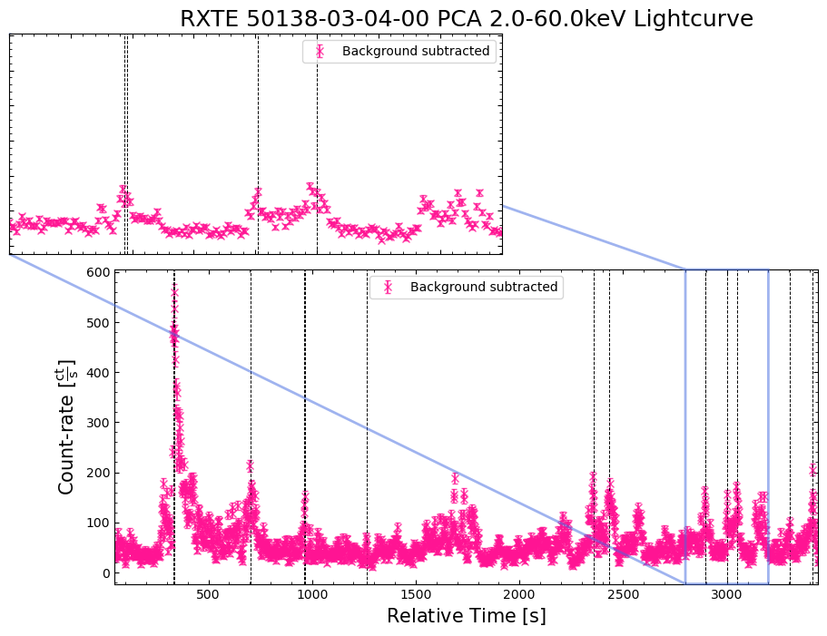
Applying wavelet transform peak finding to the whole aggregated light curve#
Following our successful test of CWT peak finding on a single light curve, we will try to apply it to the entire set of observations we have been looking at in this tutorial!
As we’re using the two-second time bin aggregated light curve set up earlier in the notebook, the single light curve we just tested on will be analyzed again, but given the speed of CWT peak-finding, that is acceptable.
We do not change the CWT peak-finding configuration parameters from the settings used for the single light curve test, given that the results seemed to be a promising start.
Extracting the count-rate and time (as seconds from reference time, and as datetimes) for each data point in the two-second time bin AggregateLightCurve object is straightforward, as is running the CWT peak-finding algorithm again:
wt_agg_demo_cr, wt_agg_demo_cr_err, wt_agg_demo_datetime, wt_agg_demo_ch_id = (
    burst_id_demo_agg_lc.get_data(date_time=True)
)
wt_agg_demo_time = burst_id_demo_agg_lc.get_data(date_time=False)[2]

# Running the peak finder on the whole aggregated light curve
wt_agg_lc_demo_bursts = find_peaks_cwt(wt_agg_demo_cr, [2, 5], min_snr=3)
Storing peak information in a Pandas DataFrame#
If this were a ‘real’ analysis, we would likely want to write the peak finding results to disk, so that they exist outside of memory in a more permanent form.
Here we will place the time and datetime of identified peaks into a Pandas DataFrame, alongside the count rate and count rate uncertainty of the data point identified as a peak, and the ID of the time chunk (which can be linked to an observation) the peak occurred during.
As well as making it easy to save this information to disk (using the to_csv()
method), the new dataframe also provides a nice way of interacting with the data
within this notebook:
# Extract useful information for each data point identified as a peak
rel_tc_ids = wt_agg_demo_ch_id[wt_agg_lc_demo_bursts]
rel_datetimes = wt_agg_demo_datetime[wt_agg_lc_demo_bursts]
rel_times = wt_agg_demo_time[wt_agg_lc_demo_bursts]
rel_crs = wt_agg_demo_cr[wt_agg_lc_demo_bursts].value
rel_cr_errs = wt_agg_demo_cr_err[wt_agg_lc_demo_bursts].value

# Set up the data and column names required to declare the dataframe
out_data = np.vstack([rel_tc_ids, rel_datetimes, rel_times, rel_crs, rel_cr_errs]).T
out_cols = ["time_chunk_id", "burst_datetime", "burst_time", "burst_cr", "burst_cr_err"]

# Make and save the dataframe
wt_agg_lc_demo_burst_res = pd.DataFrame(out_data, columns=out_cols)
wt_agg_lc_demo_burst_res.to_csv("cwt_peak_info.csv", index=False)

# We will examine the dataframe in Jupyter as well
wt_agg_lc_demo_burst_res
| time_chunk_id | burst_datetime | burst_time | burst_cr | burst_cr_err | |
|---|---|---|---|---|---|
| 0 | 0 | 2000-07-13 04:45:11.562431 | 206081055.378431 | 223.060604 | 11.389885 |
| 1 | 0 | 2000-07-13 04:55:33.562431 | 206081677.378431 | 331.641458 | 13.629187 |
| 2 | 0 | 2000-07-13 05:03:45.562431 | 206082169.378431 | 1088.23267 | 24.031044 |
| 3 | 0 | 2000-07-13 05:03:47.562431 | 206082171.378431 | 902.114175 | 21.919986 |
| 4 | 1 | 2000-07-13 17:57:31.562431 | 206128595.378431 | 379.813874 | 14.583534 |
| ... | ... | ... | ... | ... | ... |
| 498 | 57 | 2010-10-18 15:45:53.562429 | 530034299.378429 | 1710.659429 | 30.096882 |
| 499 | 57 | 2010-10-18 15:56:59.562429 | 530034965.378429 | 1698.160325 | 29.972881 |
| 500 | 57 | 2010-10-18 16:00:37.562429 | 530035183.378429 | 1681.672984 | 29.845354 |
| 501 | 57 | 2010-10-18 16:10:25.562429 | 530035771.378429 | 1504.303014 | 28.374562 |
| 502 | 57 | 2010-10-18 16:10:31.562429 | 530035777.378429 | 1538.253902 | 28.673094 |
503 rows × 5 columns
Exploring T5X2 properties at potential burst times#
We now have a set of times that represent what we think might be X-ray bursts from T5X2! Whether we arrived at them by manual inspection, or some automatic method, at this point we might want to make a simple examination of some of T5X2’s properties at the times of the potential bursts.
As this demonstration is primarily about RXTE light curves, we will focus on what insights we can draw from the products we already have available. If you were performing a full scientific analysis, you might want to consider ‘time resolved spectroscopy’ (spectra are extracted from within a specific time period of an observation).
Count rates at potential burst times#
Our first step is to examine the distribution of count rates (within the 2–60 keV band that the high-time-resolution light curves were generated within) at the times identified by the peak-finding method.
T5X2 is a complex X-ray emitter, and work by M. Linares et al. (2012) found that the bursting caused by accretion of material onto the neutron star evolved over the course of their RXTE observations. One of the most significant effects (and a key finding of their study) was that the persistent X-ray emission (the ‘base’ count rate when a burst is not occurring) increases as the bursts become more frequent.
This is indicative of a continuous process causing increased X-ray emission, fueled by a reservoir of material built up from the high accretion rate onto T5X2, and only partially consumed by X-ray bursts from the neutron star.
As such, we might wonder if the distribution of count-rates at potential burst times (defined using CWT peak finding in this case) is multi-modal, reflecting the different levels of persistent X-ray emission at different stages in T5X2’s accretion?
Looking at this distribution, we can see that there appear to be at least two distinct populations of bursts, at least when considering the burst-count-rates. This could represent two different modes of accretion and bursting, just as was seen by M. Linares et al. (2012).
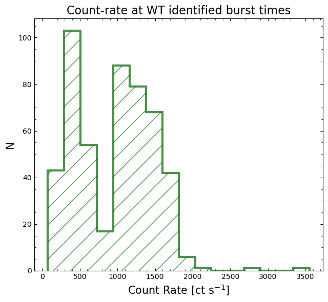
Hardness ratios at potential burst times#
Given the different astrophysical processes that appear to be driving the persistent and bursting X-ray emission by T5X2, it would also be interesting to look at the hardness ratio of the emission at the potential burst times.
We discussed hardness ratios in the previous section, calculating and visualizing a ‘hardness curve’ from our newly generated custom-energy-band light curves. Here we will pull in the unique information that those light curves contain to help paint a picture of what T5X2 might be doing.
Unfortunately, we were only able to generate light curves within specific energy bands with a time resolution of 16 seconds. This is a hard limitation of the RXTE-PCA instrument, as the ‘Standard-1’ data mode we used to make our high-time-resolution (two-second time bin in this case) contains no spectral information at all.
To determine the hardness ratio at our potential burst times, we will have to compromise and interpolate the much coarser 16-second binning of the hardness curve to our peak detection times. Doing this without further thought is acceptable because this is a demonstration, but you should consider the potential measurement effects interpolation could produce for your own science case.
Once again, using the 2–10 keV light curves as the soft band, and the 10–30 keV as the hard band, we interpolate the hardness ratio at every time step of the two-second time resolution light curves. Then the interpolated hardness ratio at the time of each potential burst is extracted:
lo_en_demo_agg_data = agg_gen_en_bnd_lcs["2.0-10.0keV"].get_data()
lo_en_demo_agg_cr = lo_en_demo_agg_data[0]
lo_en_demo_agg_time = lo_en_demo_agg_data[2]

hi_en_demo_agg_data = agg_gen_en_bnd_lcs["10.0-30.0keV"].get_data()
hi_en_demo_agg_cr = hi_en_demo_agg_data[0]
hi_en_demo_agg_time = hi_en_demo_agg_data[2]

# Calculate the hardness ratio for all data points in the 16-second time bin
#  custom-energy-band light curves
agg_lc_hard_rat = (hi_en_demo_agg_cr - lo_en_demo_agg_cr) / (
    hi_en_demo_agg_cr + lo_en_demo_agg_cr
)

# Now we interpolate the hardness curve onto the time grid of the high-time
#  resolution light curve
wt_agg_lc_demo_interp_hard = np.interp(
    wt_agg_demo_time, lo_en_demo_agg_time, agg_lc_hard_rat
)

wt_agg_lc_demo_burst_hard = wt_agg_lc_demo_interp_hard[wt_agg_lc_demo_bursts]
wt_agg_lc_demo_burst_hard
For later ease of access, we add the interpolated hardness ratios at burst times to the peak information dataframe we created earlier:
wt_agg_lc_demo_burst_res["interp_hardness"] = wt_agg_lc_demo_burst_hard
wt_agg_lc_demo_burst_res
| time_chunk_id | burst_datetime | burst_time | burst_cr | burst_cr_err | interp_hardness | |
|---|---|---|---|---|---|---|
| 0 | 0 | 2000-07-13 04:45:11.562431 | 206081055.378431 | 223.060604 | 11.389885 | -0.382796 |
| 1 | 0 | 2000-07-13 04:55:33.562431 | 206081677.378431 | 331.641458 | 13.629187 | -0.380289 |
| 2 | 0 | 2000-07-13 05:03:45.562431 | 206082169.378431 | 1088.23267 | 24.031044 | -0.575769 |
| 3 | 0 | 2000-07-13 05:03:47.562431 | 206082171.378431 | 902.114175 | 21.919986 | -0.569407 |
| 4 | 1 | 2000-07-13 17:57:31.562431 | 206128595.378431 | 379.813874 | 14.583534 | -0.442290 |
| ... | ... | ... | ... | ... | ... | ... |
| 498 | 57 | 2010-10-18 15:45:53.562429 | 530034299.378429 | 1710.659429 | 30.096882 | -0.754274 |
| 499 | 57 | 2010-10-18 15:56:59.562429 | 530034965.378429 | 1698.160325 | 29.972881 | -0.749908 |
| 500 | 57 | 2010-10-18 16:00:37.562429 | 530035183.378429 | 1681.672984 | 29.845354 | -0.754383 |
| 501 | 57 | 2010-10-18 16:10:25.562429 | 530035771.378429 | 1504.303014 | 28.374562 | -0.753365 |
| 502 | 57 | 2010-10-18 16:10:31.562429 | 530035777.378429 | 1538.253902 | 28.673094 | -0.755187 |
503 rows × 6 columns
Now that hardness ratios at potential burst times have been calculated, we can plot their distribution (just as we did for count-rate), as well as how they compare to the count-rate at the time of each potential burst.
We also include the relationship between the count-rate and interpolated ratio for every data point in the two-second time-resolution aggregated light curve (right hand panel), to give us an idea of their overall relationship.
There appear to be at least two distinct populations of bursts, in terms of their hardness ratio; one with a median hardness of ~-0.5, and another, softer, population with a median hardness of ~-0.75.
The relationship of potential burst hardness to count-rate is also interesting, with a complex morphology that could be due to at least two different processes driving the persistent and bursting X-ray emission by T5X2. The softer (more negative hardness ratio) bursts appear to have a minimal dependence on the count rate, whereas the harder segment of the hardness ratio distribution seems to become softer with increasing count rate.
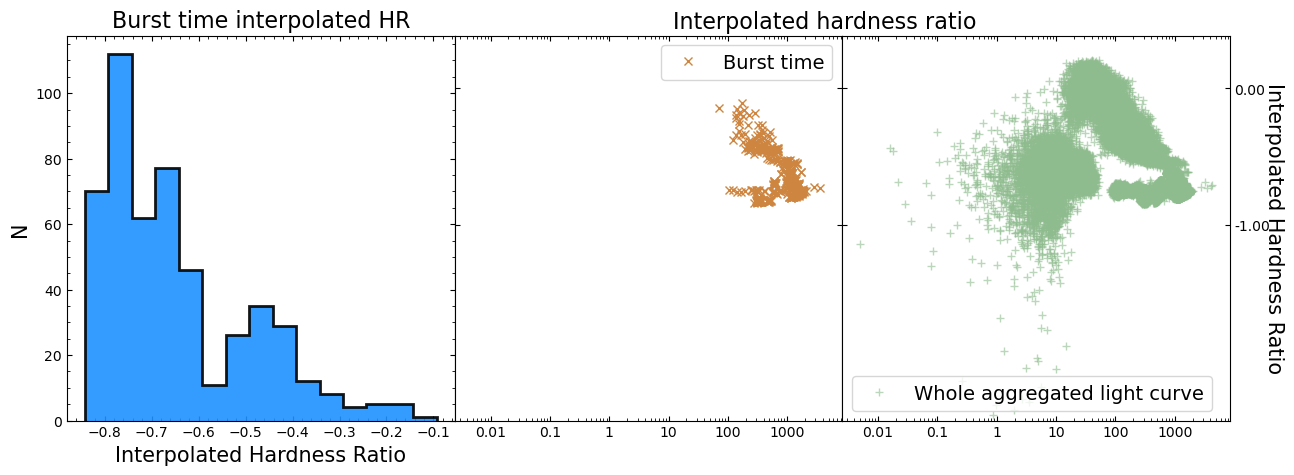
Visualizing light curves of potential bursts with hardness information#
We can also plot some of the light curves, with potential burst times highlighted, and include the interpolated hardness of the emission at burst time, to place the hardness information in context.
A subset of light curves is selected, chosen to show some interesting features and highlight the performance of the peak-finding algorithm.
As the light curves will be plotted on separate figures, but we want a consistent hardness color scale throughout, we set up a matplotlib color mapper that will take a hardness ratio value and return a color. It is normalized using the minimum and maximum burst hardness ratios of all the selected light curves.
burst_sel_mask = wt_agg_lc_demo_burst_res["time_chunk_id"] > 45
subset_wt_agg_lc_demo_burst_res = wt_agg_lc_demo_burst_res[burst_sel_mask]
subset_wt_agg_interp_burst_hardness = wt_agg_lc_demo_burst_hard[burst_sel_mask]

# We want to normalise this colourmap to our specific data range
norm = Normalize(
    vmin=subset_wt_agg_interp_burst_hardness.min(),
    vmax=subset_wt_agg_interp_burst_hardness.max(),
)
# Now a mapper can be constructed so that we can take that information about
#  the cmap and normalisation and use it with our data to calculate colours
cmap_mapper = cm.ScalarMappable(norm=norm, cmap="turbo")
# This calculates the colours
colours = cmap_mapper.to_rgba(subset_wt_agg_interp_burst_hardness)
Now we plot the selected light curves, with vertical lines indicating a potential burst, and the color of the line communicating the interpolated hardness ratio:
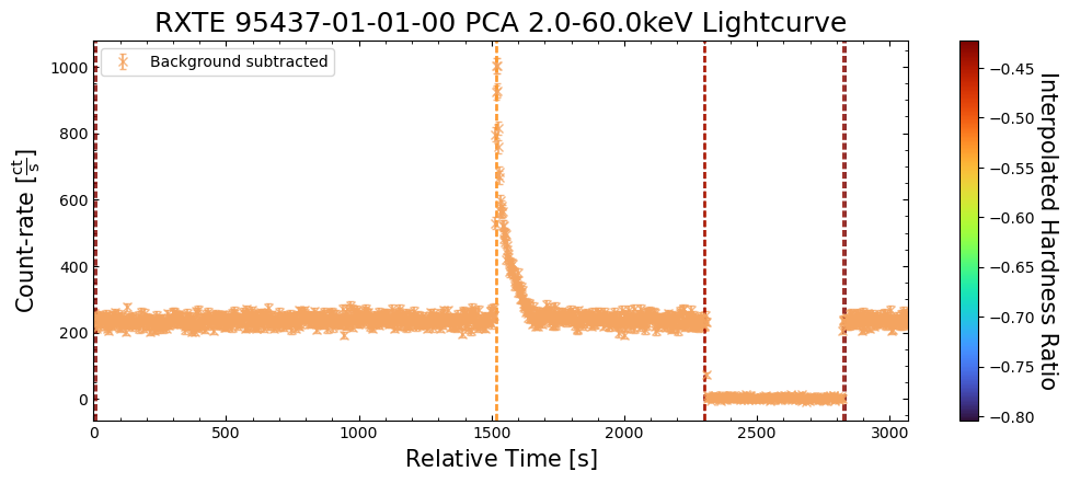
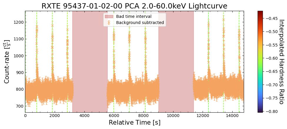
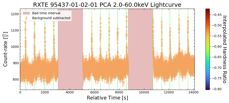
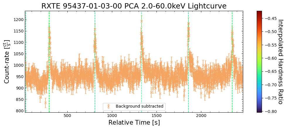
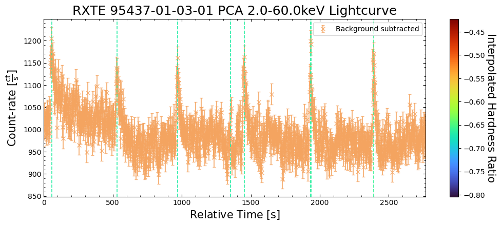
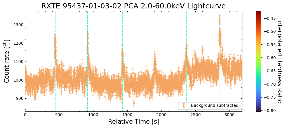
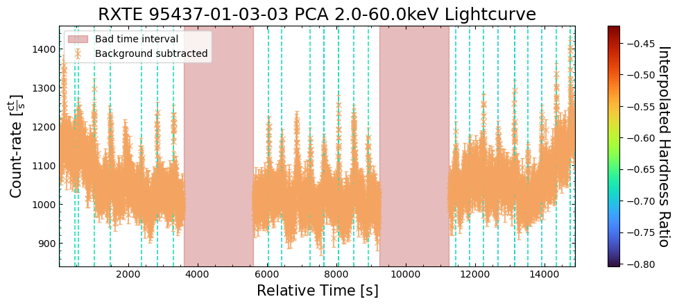
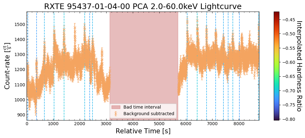
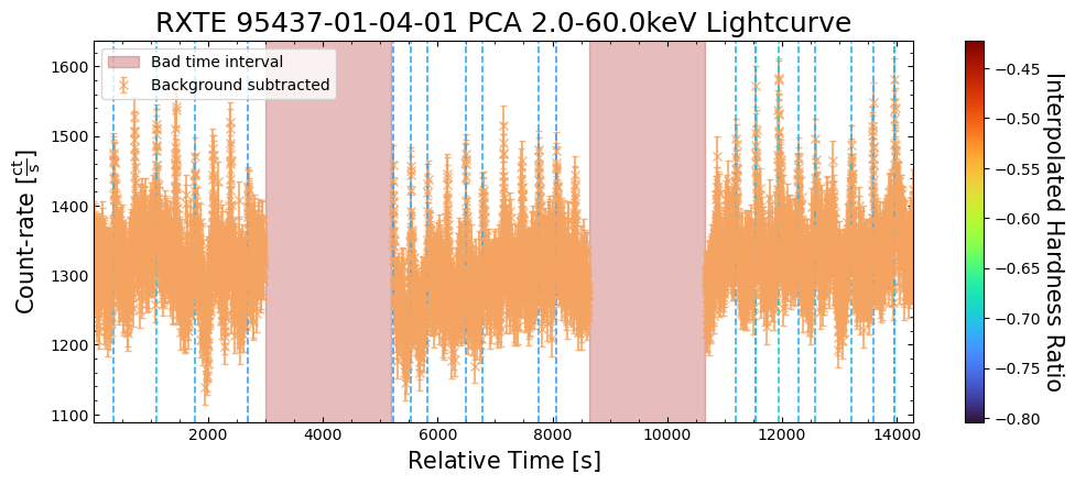
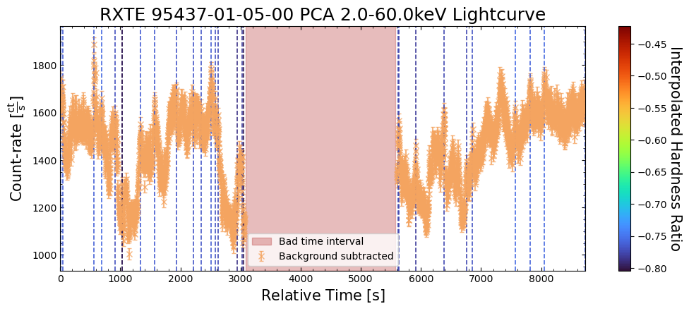
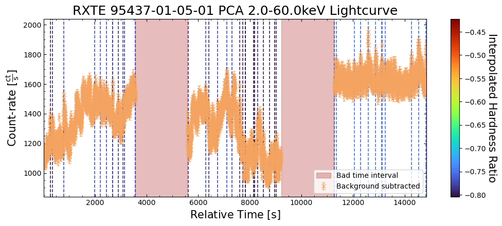
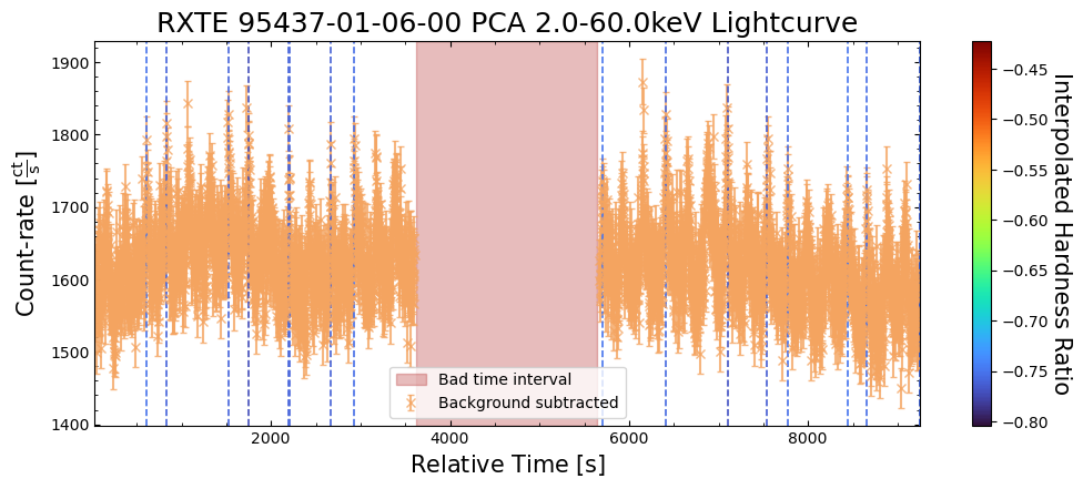
Number and frequency of potential bursts#
The number of bursts per unit time is another quantity that might be interesting to look at, as there are several potential questions it might answer. For instance:
Does the burst frequency stay constant across our observations of T5X2, or does it increase as we move into the phase of a continuous process increasing the base emission of T5X2?
As it seems there might be two distinct populations of bursts (in terms of their hardness ratio, and its relationship to count-rate), does the frequency of soft and hard bursts change over the course of our observations?
We can use our peak-finding results, alongside information extracted from the light curves, to get an idea of the potential burst frequency.
How many peaks did we find in each time chunk?#
To calculate the burst frequency, we need to start by determining how many bursts were identified during each ‘time chunk’ of our aggregated light curve.
This is made easy by our previous decision to store the burst information in
a Pandas dataframe. We can use the value_counts() method of “time_chunk_id”
column to count how many times each unique time chunk ID appears in that
column (recall that every row represents a potential burst).
The output of this is a Pandas Series with “time_chunk_id” index values and the number
of bursts with that time chunk ID as values.
We then order the series from lowest to highest time chunk ID:
burst_per_chunk = wt_agg_lc_demo_burst_res["time_chunk_id"].value_counts()
burst_per_chunk = burst_per_chunk.sort_index()
burst_per_chunk.index = burst_per_chunk.index.astype(int)
burst_per_chunk
time_chunk_id
0      4
1      8
2      1
3      7
4     13
5      2
6      2
7      2
8     11
9      7
10    18
11    21
12     6
13     5
14     4
15    13
16     7
17     2
18     7
19    17
20     4
21     9
22     3
23     5
25    13
26     3
27     5
30     5
31     2
33     1
34     2
43    13
44    45
46     8
47    18
48    26
49    10
50     8
51     9
52    29
53    17
54    21
55    30
56    43
57    17
Name: count, dtype: int64
The number of bursts detected per time chunk varies significantly, with some time chunk IDs not even represented in the dataframe (meaning no peaks were detected).
We cannot draw too many conclusions from this yet, though, as the time chunks are not guaranteed to be of equal length. Our next step has to be to calculate the number of bursts per second for each time chunk.
Calculating the frequency of bursts#
In order to calculate the frequency of burst occurrence, we need to know the length
of time represented by each time chunk. This is easy to extract (using
the time_chunk_lengths property) from the two-second time resolution
AggregateLightCurve object we set up earlier, when we generated those light curves.
Knowing the lengths of time chunks isn’t enough by itself, though, as there is no guarantee that we have data for the entire time period covered by a particular time chunk. Perhaps there were issues with the detector, or the data from part of the observation did not pass our screening criteria - either way, we can’t include such time periods, as we may underestimate the burst frequency.
The good-time-intervals of each light curve (GTIs) will tell us whether there are any time periods that we shouldn’t include in our total time chunk length determination. GTI information is loaded in from light curve files, if available, and can again be accessed through the AggregateLightCurve object.
In this instance, we can use the time_chunk_good_fractions() method of AggregateLightCurve to
retrieve the fraction of each time chunk that is within the GTIs of its light curve.
Multiplying the time chunk lengths by this fraction will give us the actual length of time we should divide the number of bursts by to get the burst frequency:
time_chunk_size = (
    burst_id_demo_agg_lc.time_chunk_lengths
    * burst_id_demo_agg_lc.time_chunk_good_fractions()
)

time_chunk_peak_freq = np.zeros(time_chunk_size.shape)
time_chunk_peak_freq[burst_per_chunk.index.values] = (
    burst_per_chunk.values / time_chunk_size[burst_per_chunk.index.values]
)

time_chunk_peak_freq
array([0.00246305, 0.00462963, 0.00099602, 0.00209205, 0.00377468,
       0.00068823, 0.00058997, 0.00084674, 0.00308989, 0.00202781,
       0.005625  , 0.00469379, 0.00129983, 0.00261233, 0.00208333,
       0.00102783, 0.00197294, 0.00104167, 0.00368809, 0.00332811,
       0.00294551, 0.00439453, 0.00089874, 0.00163613, 0.        ,
       0.00380117, 0.00086856, 0.00092353, 0.        , 0.        ,
       0.00216076, 0.00074405, 0.        , 0.00041118, 0.00067935,
       0.        , 0.        , 0.        , 0.        , 0.        ,
       0.        , 0.        , 0.        , 0.03494624, 0.01365291,
       0.        , 0.00260417, 0.00178678, 0.00257426, 0.00400641,
       0.002886  , 0.00281955, 0.00266055, 0.00274194, 0.00207428,
       0.00479386, 0.00397559, 0.00235066])
We can now plot the overall distribution of peak detection (which is hopefully correlated with burst) frequencies. The majority of our time chunks appear to not have any bursts detected, which could be a real finding, or a limitation of the automatic peak-finding algorithm/configuration.
Disregarding those with zero bursts, the distribution of peak detection frequency peaks at around 0.003 Hz, or 3 bursts per kilosecond. We also note the presence of some outliers with much higher peak detection frequencies.
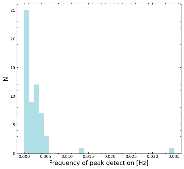
Does the frequency of peak identification evolve with time?#
We have the frequency of peak detection for each time chunk, and so we can plot it against the time chunk central time in order to see if the peak detection frequency changes over the course of our observations.
First, we calculate the time chunk central times, using Python datetime objects because matplotlib can be easily configured to display datetimes as axis labels:
datetime_chunk_halfwidths = (
    np.diff(burst_id_demo_agg_lc.datetime_chunks, axis=1).flatten() / 2
)
datetime_chunk_centers = (
    burst_id_demo_agg_lc.datetime_chunks[:, 0] + datetime_chunk_halfwidths
)
Then we can make the figure! As we are covering a time period of nearly ten years, and we are using a continuous x-axis, the data points are very close together and somewhat hard to interpret. As such, we include inset zooms into time-periods of interest.
We don’t see a dramatic difference in the peak detection frequencies at different times, though the frequencies on the right-hand side of the plot, from 2010, seem to have more consistent peak detection frequencies than those from 2001.
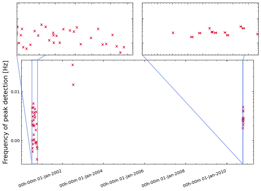
Does the hardness ratio of potential bursts evolve with time?#
Considering that we may have identified two populations of bursts with different hardness ratios, we can attempt to see if the occurrence frequency of ‘softer’ and ‘harder’ bursts changes over the course of our observations.
Based on the potential burst hardness ratio distribution visualization we created earlier, we choose a boundary of -0.6 to split the bursts into ‘softer’ (less than -0.6) and ‘harder’ (greater than -0.6) groups.
We follow the same procedure as before to calculate the potential burst frequency, first for the ‘harder’ bursts:
hard_burst_res = wt_agg_lc_demo_burst_res[
    wt_agg_lc_demo_burst_res["interp_hardness"] >= -0.6
]
hard_burst_per_chunk = hard_burst_res["time_chunk_id"].value_counts()
hard_burst_per_chunk = hard_burst_per_chunk.sort_index()
hard_burst_per_chunk.index = hard_burst_per_chunk.index.astype(int)

time_chunk_hard_peak_freq = np.zeros(time_chunk_size.shape)
time_chunk_hard_peak_freq[hard_burst_per_chunk.index.values] = (
    hard_burst_per_chunk.values / time_chunk_size[hard_burst_per_chunk.index.values]
)
Then for the ‘softer’ bursts:
soft_burst_res = wt_agg_lc_demo_burst_res[
    wt_agg_lc_demo_burst_res["interp_hardness"] < -0.6
]
soft_burst_per_chunk = soft_burst_res["time_chunk_id"].value_counts()
soft_burst_per_chunk = soft_burst_per_chunk.sort_index()
soft_burst_per_chunk.index = soft_burst_per_chunk.index.astype(int)

time_chunk_soft_peak_freq = np.zeros(time_chunk_size.shape)
time_chunk_soft_peak_freq[soft_burst_per_chunk.index.values] = (
    soft_burst_per_chunk.values / time_chunk_size[soft_burst_per_chunk.index.values]
)
The distributions of potential burst frequency for the softer and harder bursts seem fairly similar:
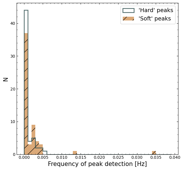
When we view the ‘harder’ and ‘softer’ burst frequencies as a function of time, however, we see a stark division between the two sets of frequencies on the plot.
We observe that most of the time chunks with a non-zero ‘hard’ (>-0.6) burst frequency have a ‘soft’ (<=-0.6) burst frequency of zero, and vice versa.
Not only that, but most of the non-zero ‘hard’ burst frequencies are found in the earliest observations, and then most of the subsequent time chunks only have non-zero ‘soft’ burst frequencies.
This may indicate that there is an evolution of the burst hardness ratio over time, though more exploration of the data, the techniques we use, and the choice of ‘hardness’ boundary would be required to confidently state this.
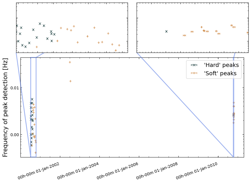
About this notebook#
Author: David J Turner, HEASARC Staff Scientist.
Author: Tess Jaffe, HEASARC Chief Archive Scientist.
Updated On: 2026-02-03
Additional Resources#
NASA press release on RXTE observations of T5X2
HEASARC discussion of RXTE-PCA screening and filtering
HEASARC RXTE-PCA energy-channel conversion table
Acknowledgements#
References#
M. Linares et al. (2012) - Millihertz Quasi-periodic Oscillations and Thermonuclear Bursts from Terzan 5: A Showcase of Burning Regimes
M. Maier et al. (2024) - Systematic review of the effects of decision fatigue in healthcare professionals on medical decision-making