Exploring RXTE spectral observations of Eta Car#
Learning Goals#
By the end of this tutorial, you will:
Know how to find and use observation tables hosted by HEASARC.
Be able to search for RXTE observations of a named source.
Understand how to access RXTE spectra stored in the HEASARC S3 bucket.
Be capable of downloading and visualizing retrieved spectra.
Perform basic spectral fits and explore how spectral properties change with time.
Use simple machine learning techniques to perform a model-independent analysis of the spectral data.
Introduction#
This notebook demonstrates an analysis of archival Rossi X-ray Timing Explorer (RXTE) Proportional Counter Array (PCA) data, particularly spectra of Eta Car.
The RXTE archive contains standard data products that can be used without re-processing the data, which are summarized in this description of standard RXTE data products.
We find all the standard spectra and then load, visualize, and fit them with PyXspec.
Inputs#
The name of the source we are going to explore using archival RXTE observations - Eta Car.
Outputs#
Downloaded source and background spectra.
Downloaded spectral response files.
Visualization of all spectra and fitted spectral models.
A figure showing powerlaw model parameter distributions from all spectral fits.
A figure showing how fitted model parameters vary with time.
Runtime#
As of 16th January 2026, this notebook takes ~3 minutes to run to completion on Fornax, using the ‘small’ server with 8GB RAM/ 2 cores.
Imports & Environments#
We need the following Python modules:
import contextlib
import os

import astropy.io.fits as fits
import matplotlib.dates as mdates
import matplotlib.pyplot as plt
import numpy as np
import xspec as xs
from astropy.coordinates import SkyCoord
from astropy.time import Time, TimeDelta
from astropy.units import Quantity
from astroquery.heasarc import Heasarc
from cycler import cycler
from matplotlib.ticker import FuncFormatter
from s3fs import S3FileSystem
from sklearn.cluster import DBSCAN
from sklearn.decomposition import PCA
from sklearn.manifold import TSNE
from sklearn.preprocessing import StandardScaler
from tqdm import tqdm
from umap import UMAP
/opt/envs/heasoft/lib/python3.12/site-packages/tqdm/auto.py:21: TqdmWarning: IProgress not found. Please update jupyter and ipywidgets. See https://ipywidgets.readthedocs.io/en/stable/user_install.html
  from .autonotebook import tqdm as notebook_tqdm
Global Setup#
Functions#
Constants#
Configuration#
The only configuration we do is to set up the root directory where we will store downloaded data.
1. Finding the data#
To identify the relevant RXTE data, we could use Xamin, the HEASARC web portal, the Virtual Observatory (VO) python client pyvo, or the Astroquery module (our choice for this demonstration).
Using Astroquery to find the HEASARC table that lists all of RXTE’s observations#
Using the Heasarc object from Astroquery, we can easily search through all of HEASARC’s catalog holdings. In this
case we need to find what we refer to as a ‘master’ catalog/table, which summarizes all RXTE observations present in
our archive. We can do this by passing the master=True keyword argument to the list_catalogs method.
table_name = Heasarc.list_catalogs(keywords="xte", master=True)[0]["name"]
table_name
np.str_('xtemaster')
Identifying RXTE observations of Eta Car#
Now that we have identified the HEASARC table that contains summary information about all of RXTE’s observations, we’re going to search it for observations of Eta Car.
For convenience, we pull the coordinate of Eta Car from the Strasbourg astronomical Data Center (CDS) name resolver functionality built into Astropy’s
SkyCoord class.
Caution
You should always carefully vet the positions you use in your own work!
# Get the coordinate for Eta Car
pos = SkyCoord.from_name("Eta Car")
pos
<SkyCoord (ICRS): (ra, dec) in deg
    (161.2647742, -59.6844309)>
Then we can use the query_region method of Heasarc to search for observations with a central coordinate that
falls within a radius of \(0.2^{\prime}\) of Eta Car.
Hint
Each HEASARC catalog has its own default search radius, but we select \(0.2^{\prime}\) to limit the number of results. You should carefully consider the search radius you use for your own science case!
valid_obs = Heasarc.query_region(
    pos, catalog=table_name, radius=Quantity(0.2, "arcmin")
)
valid_obs
| obsid | prnb | status | pi_lname | pi_fname | target_name | ra | dec | time | duration | exposure | __row |
|---|---|---|---|---|---|---|---|---|---|---|---|
| deg | deg | d | s | s | |||||||
| object | int32 | object | object | object | object | float64 | float64 | float64 | float64 | float64 | object |
| 94002-01-15-00 | 94002 | archived | TOO | PUBLIC | ETA_CAR | 161.2650 | -59.6845 | 55000.4322 | 2518 | 1197 | 16751 |
| 93002-01-17-00 | 93002 | archived | CORCORAN | MICHAEL | ETA_CAR | 161.2650 | -59.6845 | 54398.83492 | 2179 | 924 | 16752 |
| 93002-02-52-00 | 93002 | archived | CORCORAN | MICHAEL | ETA_CAR | 161.2650 | -59.6845 | 54808.7048 | 1582 | 905 | 16753 |
| 93002-02-53-00 | 93002 | archived | CORCORAN | MICHAEL | ETA_CAR | 161.2650 | -59.6845 | 54810.66671 | 1510 | 829 | 16754 |
| 93002-02-54-00 | 93002 | archived | CORCORAN | MICHAEL | ETA_CAR | 161.2650 | -59.6845 | 54812.85572 | 1430 | 927 | 16755 |
| 93002-01-47-00 | 93002 | archived | CORCORAN | MICHAEL | ETA_CAR | 161.2650 | -59.6845 | 54606.98389 | 3246 | 863 | 16756 |
| 93002-02-55-00 | 93002 | archived | CORCORAN | MICHAEL | ETA_CAR | 161.2650 | -59.6845 | 54814.29519 | 2168 | 771 | 16757 |
| 93002-02-56-00 | 93002 | archived | CORCORAN | MICHAEL | ETA_CAR | 161.2650 | -59.6845 | 54816.35667 | 2442 | 885 | 16758 |
| 93002-02-57-00 | 93002 | archived | CORCORAN | MICHAEL | ETA_CAR | 161.2650 | -59.6845 | 54818.31775 | 2273 | 830 | 16759 |
| ... | ... | ... | ... | ... | ... | ... | ... | ... | ... | ... | ... |
| 93002-02-45-00 | 93002 | archived | CORCORAN | MICHAEL | ETA_CAR | 161.2650 | -59.6845 | 54794.04643 | 2080 | 853 | 17059 |
| 93002-01-32-00 | 93002 | archived | CORCORAN | MICHAEL | ETA_CAR | 161.2650 | -59.6845 | 54502.15576 | 2869 | 923 | 17060 |
| 93002-02-46-00 | 93002 | archived | CORCORAN | MICHAEL | ETA_CAR | 161.2650 | -59.6845 | 54796.9229 | 1269 | 957 | 17061 |
| 93002-02-47-00 | 93002 | archived | CORCORAN | MICHAEL | ETA_CAR | 161.2650 | -59.6845 | 54798.88473 | 1992 | 951 | 17062 |
| 93002-02-48-00 | 93002 | archived | CORCORAN | MICHAEL | ETA_CAR | 161.2650 | -59.6845 | 54800.43516 | 1740 | 943 | 17063 |
| 93002-02-49-00 | 93002 | archived | CORCORAN | MICHAEL | ETA_CAR | 161.2650 | -59.6845 | 54803.07797 | 1680 | 1077 | 17064 |
| 93002-02-50-00 | 93002 | archived | CORCORAN | MICHAEL | ETA_CAR | 161.2650 | -59.6845 | 54804.38447 | 2856 | 882 | 17065 |
| 93002-02-51-00 | 93002 | archived | CORCORAN | MICHAEL | ETA_CAR | 161.2650 | -59.6845 | 54806.15838 | 1422 | 888 | 17066 |
| 94418-01-01-00 | 94418 | archived | TOO | PUBLIC | ETA_CAR | 161.2650 | -59.6840 | 54899.76288 | 1934 | 1017 | 17067 |
Alternatively, if you wished to place extra constraints on the search, you could use the more complex query_tap method
to pass a full Astronomical Data Query Language (ADQL) query. Using ADQL allows you to be much more flexible but in
many cases may not be necessary.
This demonstration runs the same spatial query as before but also includes a stringent exposure time requirement; you might do this to try and only select the highest signal-to-noise observations.
Note that we call the to_table method on the result of the query to convert the result into an Astropy table, which
is the form required to pass to the locate_data method (see the next section).
query = (
    "SELECT * "
    "from {c} as cat "
    "where contains(point('ICRS',cat.ra,cat.dec), circle('ICRS',{ra},{dec},0.0033))=1 "
    "and cat.exposure > 1200".format(ra=pos.ra.value, dec=pos.dec.value, c=table_name)
)

alt_obs = Heasarc.query_tap(query).to_table()
alt_obs
| __row | pi_lname | pi_fname | pi_no | prnb | cycle | subject_category | target_name | time_awarded | ra | dec | priority | tar_no | obsid | time | duration | exposure | status | scheduled_date | observed_date | processed_date | archived_date | hexte_anglea | hexte_angleb | hexte_dwella | hexte_dwellb | hexte_energya | hexte_energyb | hexte_modea | hexte_modeb | pca_config1 | pca_config2 | pca_config3 | pca_config4 | pca_config5 | pca_config6 | lii | bii | __x_ra_dec | __y_ra_dec | __z_ra_dec |
|---|---|---|---|---|---|---|---|---|---|---|---|---|---|---|---|---|---|---|---|---|---|---|---|---|---|---|---|---|---|---|---|---|---|---|---|---|---|---|---|---|
| s | deg | deg | d | s | s | d | d | d | d | deg | deg | |||||||||||||||||||||||||||||
| object | object | object | int32 | int32 | int16 | object | object | float64 | float64 | float64 | int16 | int16 | object | float64 | float64 | float64 | object | float64 | float64 | int32 | int32 | object | object | object | object | object | object | object | object | object | object | object | object | object | object | float64 | float64 | float64 | float64 | float64 |
| 16769 | CORCORAN | MICHAEL | 196 | 93002 | 12 | STARS | ETA_CAR | 85000.0 | 161.2650 | -59.6845 | 1 | 2 | 93002-02-66-00 | 54836.05479 | 2428 | 1267 | archived | 54836.05479 | 54836.05479 | 54845 | 55211 | DEFAULT | DEFAULT | DEFAULT | DEFAULT | DEFAULT | DEFAULT | E_8US_256_DX1F | E_8US_256_DX1F | STANDARD1 | STANDARD2 | GOODXENON1_2S | GOODXENON2_2S | IDLE | IDLE | 287.5969 | -0.6295 | 0.162125023877781 | -0.478016026673964 | -0.863259031157778 |
| 16771 | CORCORAN | MICHAEL | 196 | 93002 | 12 | STARS | ETA_CAR | 85000.0 | 161.2650 | -59.6845 | 1 | 2 | 93002-02-68-00 | 54840.44851 | 2842 | 1335 | archived | 54840.44851 | 54840.44851 | 54850 | 55218 | DEFAULT | DEFAULT | DEFAULT | DEFAULT | DEFAULT | DEFAULT | E_8US_256_DX1F | E_8US_256_DX1F | STANDARD1 | STANDARD2 | GOODXENON1_2S | GOODXENON2_2S | IDLE | IDLE | 287.5969 | -0.6295 | 0.162125023877781 | -0.478016026673964 | -0.863259031157778 |
| 16777 | CORCORAN | MICHAEL | 196 | 93002 | 12 | STARS | ETA_CAR | 85000.0 | 161.2650 | -59.6845 | 1 | 2 | 93002-02-73-00 | 54850.24669 | 3308 | 1651 | archived | 54850.24669 | 54850.24669 | 54859 | 55225 | DEFAULT | DEFAULT | DEFAULT | DEFAULT | DEFAULT | DEFAULT | E_8US_256_DX1F | E_8US_256_DX1F | STANDARD1 | STANDARD2 | GOODXENON1_2S | GOODXENON2_2S | IDLE | IDLE | 287.5969 | -0.6295 | 0.162125023877781 | -0.478016026673964 | -0.863259031157778 |
| 16789 | CORCORAN | MICHAEL | 196 | 93002 | 12 | STARS | ETA_CAR | 85000.0 | 161.2650 | -59.6845 | 1 | 2 | 93002-02-84-00 | 54872.22313 | 2542 | 1283 | archived | 54872.22313 | 54872.22313 | 54880 | 55247 | DEFAULT | DEFAULT | DEFAULT | DEFAULT | DEFAULT | DEFAULT | E_8US_256_DX1F | E_8US_256_DX1F | STANDARD1 | STANDARD2 | GOODXENON1_2S | GOODXENON2_2S | IDLE | IDLE | 287.5969 | -0.6295 | 0.162125023877781 | -0.478016026673964 | -0.863259031157778 |
| 16797 | TOO | PUBLIC | 0 | 94002 | 13 | STARS | ETA_CAR | 1310.0 | 161.2650 | -59.6845 | 0 | 1 | 94002-01-05-00 | 54930.46883 | 1725 | 1313 | archived | 54930.46883 | 54930.46883 | 54938 | -- | DEFAULT | DEFAULT | DEFAULT | DEFAULT | DEFAULT | DEFAULT | E_8us_256_DX1F | E_8us_256_DX1F | GOODXENON1_2S | GOODXENON2_2S | GOODVLE1_2S | STANDARD1B | STANDARD2F | GOODVLE2_2S | 287.5969 | -0.6295 | 0.162125023877781 | -0.478016026673964 | -0.863259031157778 |
| 16799 | TOO | PUBLIC | 0 | 94002 | 13 | STARS | ETA_CAR | 1210.0 | 161.2650 | -59.6845 | 0 | 1 | 94002-01-07-00 | 54944.20307 | 2695 | 1207 | archived | 54944.20307 | 54944.20307 | 54952 | -- | DEFAULT | DEFAULT | DEFAULT | DEFAULT | DEFAULT | DEFAULT | E_8us_256_DX1F | E_8us_256_DX1F | GOODXENON1_2S | GOODXENON2_2S | GOODVLE1_2S | STANDARD1B | STANDARD2F | GOODVLE2_2S | 287.5969 | -0.6295 | 0.162125023877781 | -0.478016026673964 | -0.863259031157778 |
| 16803 | CORCORAN | MICHAEL | 196 | 93002 | 12 | STARS | ETA_CAR | 65000.0 | 161.2650 | -59.6845 | 1 | 1 | 93002-01-49-00 | 54620.98435 | 2615 | 1504 | archived | 54620.98435 | 54620.98435 | 54629 | 54994 | DEFAULT | DEFAULT | DEFAULT | DEFAULT | DEFAULT | DEFAULT | E_8US_256_DX1F | E_8US_256_DX1F | STANDARD1 | STANDARD2 | GOODXENON1_2S | GOODXENON2_2S | IDLE | IDLE | 287.5969 | -0.6295 | 0.162125023877781 | -0.478016026673964 | -0.863259031157778 |
| 16804 | TOO | PUBLIC | 0 | 94002 | 13 | STARS | ETA_CAR | 1400.0 | 161.2650 | -59.6845 | 0 | 1 | 94002-01-11-00 | 54971.98391 | 2823 | 1401 | archived | 54971.98391 | 54971.98391 | 54980 | -- | DEFAULT | DEFAULT | DEFAULT | DEFAULT | DEFAULT | DEFAULT | E_8us_256_DX1F | E_8us_256_DX1F | GOODXENON1_2S | GOODXENON2_2S | GOODVLE1_2S | STANDARD1B | STANDARD2F | GOODVLE2_2S | 287.5969 | -0.6295 | 0.162125023877781 | -0.478016026673964 | -0.863259031157778 |
| 16805 | TOO | PUBLIC | 0 | 94002 | 13 | STARS | ETA_CAR | 1320.0 | 161.2650 | -59.6845 | 0 | 1 | 94002-01-12-00 | 54978.67289 | 2346 | 1320 | archived | 54978.67289 | 54978.67289 | 54986 | -- | DEFAULT | DEFAULT | DEFAULT | DEFAULT | DEFAULT | DEFAULT | E_8us_256_DX1F | E_8us_256_DX1F | GOODXENON1_2S | GOODXENON2_2S | GOODVLE1_2S | STANDARD1B | STANDARD2F | GOODVLE2_2S | 287.5969 | -0.6295 | 0.162125023877781 | -0.478016026673964 | -0.863259031157778 |
| ... | ... | ... | ... | ... | ... | ... | ... | ... | ... | ... | ... | ... | ... | ... | ... | ... | ... | ... | ... | ... | ... | ... | ... | ... | ... | ... | ... | ... | ... | ... | ... | ... | ... | ... | ... | ... | ... | ... | ... | ... |
| 16975 | CORCORAN | MICHAEL | 196 | 93002 | 12 | STARS | ETA_CAR | 65000.0 | 161.2650 | -59.6845 | 1 | 1 | 93002-01-27-00 | 54468.31416 | 2400 | 1211 | archived | 54468.31416 | 54468.31416 | 54479 | 54848 | DEFAULT | DEFAULT | DEFAULT | DEFAULT | DEFAULT | DEFAULT | E_8US_256_DX1F | E_8US_256_DX1F | STANDARD1 | STANDARD2 | GOODXENON1_2S | GOODXENON2_2S | IDLE | IDLE | 287.5969 | -0.6295 | 0.162125023877781 | -0.478016026673964 | -0.863259031157778 |
| 16983 | TOO | PUBLIC | 0 | 96002 | 15 | STARS | ETA_CAR | 1550.0 | 161.2650 | -59.6845 | 0 | 1 | 96002-01-48-00 | 55895.6681 | 2769 | 1550 | archived | 55895.6681 | 55895.6681 | 55903 | -- | DEFAULT | DEFAULT | DEFAULT | DEFAULT | DEFAULT | DEFAULT | E_8us_256_DX1F | E_8us_256_DX1F | GOODXENON1_2S | GOODXENON2_2S | GOODVLE1_2S | STANDARD1B | STANDARD2F | GOODVLE2_2S | 287.5969 | -0.6295 | 0.162125023877781 | -0.478016026673964 | -0.863259031157778 |
| 16985 | TOO | PUBLIC | 0 | 96002 | 15 | STARS | ETA_CAR | 1340.0 | 161.2650 | -59.6845 | 0 | 1 | 96002-01-50-00 | 55909.92591 | 1788 | 1339 | archived | 55909.92591 | 55909.92591 | 55917 | -- | DEFAULT | DEFAULT | DEFAULT | DEFAULT | DEFAULT | DEFAULT | E_8us_256_DX1F | E_8us_256_DX1F | GOODXENON1_2S | GOODXENON2_2S | GOODVLE1_2S | STANDARD1B | STANDARD2F | GOODVLE2_2S | 287.5969 | -0.6295 | 0.162125023877781 | -0.478016026673964 | -0.863259031157778 |
| 16993 | CORCORAN | MICHAEL | 196 | 93002 | 12 | STARS | ETA_CAR | 65000.0 | 161.2650 | -59.6845 | 1 | 1 | 93002-01-01-00 | 54286.22152 | 2484 | 1316 | archived | 54286.22152 | 54286.22152 | 54297 | 54667 | DEFAULT | DEFAULT | DEFAULT | DEFAULT | DEFAULT | DEFAULT | E_8US_256_DX1F | E_8US_256_DX1F | STANDARD1 | STANDARD2 | GOODXENON1_2S | GOODXENON2_2S | IDLE | IDLE | 287.5969 | -0.6295 | 0.162125023877781 | -0.478016026673964 | -0.863259031157778 |
| 16999 | CORCORAN | MICHAEL | 196 | 93002 | 12 | STARS | ETA_CAR | 65000.0 | 161.2650 | -59.6845 | 1 | 1 | 93002-01-57-00 | 54677.83937 | 1803 | 1234 | archived | 54677.83937 | 54677.83937 | 54685 | 55050 | DEFAULT | DEFAULT | DEFAULT | DEFAULT | DEFAULT | DEFAULT | E_8US_256_DX1F | E_8US_256_DX1F | STANDARD1 | STANDARD2 | GOODXENON1_2S | GOODXENON2_2S | IDLE | IDLE | 287.5969 | -0.6295 | 0.162125023877781 | -0.478016026673964 | -0.863259031157778 |
| 17007 | CORCORAN | MICHAEL | 196 | 93002 | 12 | STARS | ETA_CAR | 65000.0 | 161.2650 | -59.6845 | 1 | 1 | 93002-01-64-00 | 54894.6579 | 2580 | 1386 | archived | 54894.6579 | 54894.6579 | 54902 | 55267 | DEFAULT | DEFAULT | DEFAULT | DEFAULT | DEFAULT | DEFAULT | E_8US_256_DX1F | E_8US_256_DX1F | STANDARD1 | STANDARD2 | GOODXENON1_2S | GOODXENON2_2S | IDLE | IDLE | 287.5969 | -0.6295 | 0.162125023877781 | -0.478016026673964 | -0.863259031157778 |
| 17008 | CORCORAN | MICHAEL | 196 | 93002 | 12 | STARS | ETA_CAR | 65000.0 | 161.2650 | -59.6845 | 1 | 1 | 93002-01-65-00 | 54847.22777 | 1680 | 1317 | archived | 54847.22777 | 54847.22777 | 54857 | 55225 | DEFAULT | DEFAULT | DEFAULT | DEFAULT | DEFAULT | DEFAULT | E_8US_256_DX1F | E_8US_256_DX1F | STANDARD1 | STANDARD2 | GOODXENON1_2S | GOODXENON2_2S | IDLE | IDLE | 287.5969 | -0.6295 | 0.162125023877781 | -0.478016026673964 | -0.863259031157778 |
| 17015 | CORCORAN | MICHAEL | 196 | 93002 | 12 | STARS | ETA_CAR | 85000.0 | 161.2650 | -59.6845 | 1 | 2 | 93002-02-06-00 | 54716.71092 | 2739 | 1353 | archived | 54716.71092 | 54716.71092 | 54724 | 55092 | DEFAULT | DEFAULT | DEFAULT | DEFAULT | DEFAULT | DEFAULT | E_8US_256_DX1F | E_8US_256_DX1F | STANDARD1 | STANDARD2 | GOODXENON1_2S | GOODXENON2_2S | IDLE | IDLE | 287.5969 | -0.6295 | 0.162125023877781 | -0.478016026673964 | -0.863259031157778 |
| 17032 | CORCORAN | MICHAEL | 196 | 93002 | 12 | STARS | ETA_CAR | 85000.0 | 161.2650 | -59.6845 | 1 | 2 | 93002-02-21-00 | 54746.01762 | 2187 | 1375 | archived | 54746.01762 | 54746.01762 | 54754 | 55120 | DEFAULT | DEFAULT | DEFAULT | DEFAULT | DEFAULT | DEFAULT | E_8US_256_DX1F | E_8US_256_DX1F | STANDARD1 | STANDARD2 | GOODXENON1_2S | GOODXENON2_2S | IDLE | IDLE | 287.5969 | -0.6295 | 0.162125023877781 | -0.478016026673964 | -0.863259031157778 |
Using Astroquery to fetch datalinks to RXTE datasets#
We’ve already figured out which HEASARC table to pull RXTE observation information from, and then used that table to identify specific observations that might be relevant to our target source (Eta Car). Our next step is to pinpoint the exact location of files from each observation that we can use to visualize the spectral emission of our source.
Just as in the last two steps, we’re going to make use of Astroquery. The difference is, rather than dealing with tables of observations, we now need to construct ‘datalinks’ to places where specific files for each observation are stored. In this demonstration we’re going to pull data from the HEASARC ‘S3 bucket’, an Amazon-hosted open-source dataset containing all of HEASARC’s data holdings.
data_links = Heasarc.locate_data(valid_obs, "xtemaster")
data_links
| ID | access_url | sciserver | aws | content_length | error_message |
|---|---|---|---|---|---|
| byte | |||||
| object | object | str50 | str63 | int64 | object |
| ivo://nasa.heasarc/xtemaster?16751 | https://heasarc.gsfc.nasa.gov/FTP/xte/data/archive/AO13/P94002/94002-01-15-00// | /FTP/xte/data/archive/AO13/P94002/94002-01-15-00/ | s3://nasa-heasarc/xte/data/archive/AO13/P94002/94002-01-15-00/ | -- | |
| ivo://nasa.heasarc/xtemaster?16751 | https://heasarc.gsfc.nasa.gov/FTP/xte/data/archive/AO13/P94002/94002-01-15-00A// | /FTP/xte/data/archive/AO13/P94002/94002-01-15-00A/ | s3://nasa-heasarc/xte/data/archive/AO13/P94002/94002-01-15-00A/ | -- | |
| ivo://nasa.heasarc/xtemaster?16751 | https://heasarc.gsfc.nasa.gov/FTP/xte/data/archive/AO13/P94002/94002-01-15-00Z// | /FTP/xte/data/archive/AO13/P94002/94002-01-15-00Z/ | s3://nasa-heasarc/xte/data/archive/AO13/P94002/94002-01-15-00Z/ | -- | |
| ivo://nasa.heasarc/xtemaster?16751 | https://heasarc.gsfc.nasa.gov/FTP/xte/data/archive/AO13/P94002//94002-01-15-00/ | /FTP/xte/data/archive/AO13/P94002/94002-01-15-00/ | s3://nasa-heasarc/xte/data/archive/AO13/P94002/94002-01-15-00/ | -- | |
| ivo://nasa.heasarc/xtemaster?16751 | https://heasarc.gsfc.nasa.gov/FTP/xte/data/archive/AO13/P94002//94002-01/ | /FTP/xte/data/archive/AO13/P94002/94002-01/ | s3://nasa-heasarc/xte/data/archive/AO13/P94002/94002-01/ | -- | |
| ivo://nasa.heasarc/xtemaster?16752 | https://heasarc.gsfc.nasa.gov/FTP/xte/data/archive/AO12/P93002/93002-01-17-00// | /FTP/xte/data/archive/AO12/P93002/93002-01-17-00/ | s3://nasa-heasarc/xte/data/archive/AO12/P93002/93002-01-17-00/ | -- | |
| ivo://nasa.heasarc/xtemaster?16752 | https://heasarc.gsfc.nasa.gov/FTP/xte/data/archive/AO12/P93002/93002-01-17-00A// | /FTP/xte/data/archive/AO12/P93002/93002-01-17-00A/ | s3://nasa-heasarc/xte/data/archive/AO12/P93002/93002-01-17-00A/ | -- | |
| ivo://nasa.heasarc/xtemaster?16752 | https://heasarc.gsfc.nasa.gov/FTP/xte/data/archive/AO12/P93002/93002-01-17-00Z// | /FTP/xte/data/archive/AO12/P93002/93002-01-17-00Z/ | s3://nasa-heasarc/xte/data/archive/AO12/P93002/93002-01-17-00Z/ | -- | |
| ivo://nasa.heasarc/xtemaster?16752 | https://heasarc.gsfc.nasa.gov/FTP/xte/data/archive/AO12/P93002//93002-01-17-00/ | /FTP/xte/data/archive/AO12/P93002/93002-01-17-00/ | s3://nasa-heasarc/xte/data/archive/AO12/P93002/93002-01-17-00/ | -- | |
| ... | ... | ... | ... | ... | ... |
| ivo://nasa.heasarc/xtemaster?17066 | https://heasarc.gsfc.nasa.gov/FTP/xte/data/archive/AO12/P93002/93002-02-51-00A// | /FTP/xte/data/archive/AO12/P93002/93002-02-51-00A/ | s3://nasa-heasarc/xte/data/archive/AO12/P93002/93002-02-51-00A/ | -- | |
| ivo://nasa.heasarc/xtemaster?17066 | https://heasarc.gsfc.nasa.gov/FTP/xte/data/archive/AO12/P93002/93002-02-51-00Z// | /FTP/xte/data/archive/AO12/P93002/93002-02-51-00Z/ | s3://nasa-heasarc/xte/data/archive/AO12/P93002/93002-02-51-00Z/ | -- | |
| ivo://nasa.heasarc/xtemaster?17066 | https://heasarc.gsfc.nasa.gov/FTP/xte/data/archive/AO12/P93002//93002-02-51-00/ | /FTP/xte/data/archive/AO12/P93002/93002-02-51-00/ | s3://nasa-heasarc/xte/data/archive/AO12/P93002/93002-02-51-00/ | -- | |
| ivo://nasa.heasarc/xtemaster?17066 | https://heasarc.gsfc.nasa.gov/FTP/xte/data/archive/AO12/P93002//93002-02/ | /FTP/xte/data/archive/AO12/P93002/93002-02/ | s3://nasa-heasarc/xte/data/archive/AO12/P93002/93002-02/ | -- | |
| ivo://nasa.heasarc/xtemaster?17067 | https://heasarc.gsfc.nasa.gov/FTP/xte/data/archive/AO13/P94418/94418-01-01-00// | /FTP/xte/data/archive/AO13/P94418/94418-01-01-00/ | s3://nasa-heasarc/xte/data/archive/AO13/P94418/94418-01-01-00/ | -- | |
| ivo://nasa.heasarc/xtemaster?17067 | https://heasarc.gsfc.nasa.gov/FTP/xte/data/archive/AO13/P94418/94418-01-01-00A// | /FTP/xte/data/archive/AO13/P94418/94418-01-01-00A/ | s3://nasa-heasarc/xte/data/archive/AO13/P94418/94418-01-01-00A/ | -- | |
| ivo://nasa.heasarc/xtemaster?17067 | https://heasarc.gsfc.nasa.gov/FTP/xte/data/archive/AO13/P94418/94418-01-01-00Z// | /FTP/xte/data/archive/AO13/P94418/94418-01-01-00Z/ | s3://nasa-heasarc/xte/data/archive/AO13/P94418/94418-01-01-00Z/ | -- | |
| ivo://nasa.heasarc/xtemaster?17067 | https://heasarc.gsfc.nasa.gov/FTP/xte/data/archive/AO13/P94418//94418-01-01-00/ | /FTP/xte/data/archive/AO13/P94418/94418-01-01-00/ | s3://nasa-heasarc/xte/data/archive/AO13/P94418/94418-01-01-00/ | -- | |
| ivo://nasa.heasarc/xtemaster?17067 | https://heasarc.gsfc.nasa.gov/FTP/xte/data/archive/AO13/P94418//94418-01/ | /FTP/xte/data/archive/AO13/P94418/94418-01/ | s3://nasa-heasarc/xte/data/archive/AO13/P94418/94418-01/ | -- |
2. Acquiring the data#
We now know where the relevant RXTE-PCA spectra are stored in the HEASARC S3 bucket and will proceed to download them for local use.
Caution
Many workflows are being adapted to stream remote data directly into memory (RAM), rather than downloading it onto disk storage, then reading into memory - PyXspec does not yet support this way of operating, but our demonstrations will be updated when it does.
The easiest way to download data#
At this point, you may wish to simply download the entire set of files for all the observations you’ve identified.
That is easily achieved using Astroquery, with the download_data method of Heasarc, we just need to pass
the datalinks we found in the previous step.
We demonstrate this approach using the first three entries in the datalinks table, but in the following sections will demonstrate a more complicated, but targeted, approach that will let us download only the RXTE-PCA spectra and their supporting files:
Heasarc.download_data(data_links[:3], host="aws", location=ROOT_DATA_DIR)
INFO: Downloading data AWS S3 ... [astroquery.heasarc.core]
INFO: Enabling anonymous cloud data access ... [astroquery.heasarc.core]
INFO: downloading s3://nasa-heasarc/xte/data/archive/AO13/P94002/94002-01-15-00/ [astroquery.heasarc.core]
INFO: downloading s3://nasa-heasarc/xte/data/archive/AO13/P94002/94002-01-15-00A/ [astroquery.heasarc.core]
INFO: downloading s3://nasa-heasarc/xte/data/archive/AO13/P94002/94002-01-15-00Z/ [astroquery.heasarc.core]
INFO: downloading s3://nasa-heasarc/xte/data/archive/AO13/P94002/94002-01-15-00A/ [astroquery.heasarc.core]
INFO: downloading s3://nasa-heasarc/xte/data/archive/AO13/P94002/94002-01-15-00Z/ [astroquery.heasarc.core]
Downloading only RXTE-PCA spectra#
Rather than downloading all files for all our observations, we will now only fetch those that are directly relevant to what we want to do in this notebook. This method is a little more involved than using Astroquery, but it is more efficient and flexible.
We make use of a Python module called s3fs, which allows us to interact with files stored on Amazon’s S3
platform through Python commands.
We create an S3FileSystem object, which lets us interact with the S3 bucket as if it were a filesystem.
Hint
Note the anon=True argument, as attempting access to the HEASARC S3 bucket will fail without it!
s3 = S3FileSystem(anon=True)
Now we identify the specific files we want to download. The datalink table tells us the AWS S3 ‘path’ (the Uniform Resource Identifier, or URI) to each observation’s data directory, the RXTE documentation tells us that the automatically generated data products are stored in a subdirectory called ‘stdprod’, and the RXTE Guest Observer Facility (GOF) standard product guide shows us that PCA spectra and supporting files are named as:
xp{ObsID}_s2.pha - the spectrum automatically generated for the target of the RXTE observation.
xp{ObsID}_b2.pha - the background spectrum companion to the source spectrum.
xp{ObsID}.rsp - the supporting file that defines the response curve (sensitivity over energy range) and redistribution matrix (a mapping of channel to energy) for the RXTE-PCA instrument during the observation.
We set up patterns for these three files for each datalink entry, and then use the expand_path method of
our previously set-up S3 filesystem object to find all the files that match the pattern. This is useful because the
RXTE datalinks we found might include sections of a particular observation that do not have standard products
generated, for instance, the slewing periods before/after the telescope was aligned on target.
all_file_patt = [
    os.path.join(base_uri, "stdprod", fp)
    for base_uri in data_links["aws"].value
    for fp in ["xp*_s2.pha*", "xp*_b2.pha*", "xp*.rsp*"]
]

val_file_uris = s3.expand_path(all_file_patt)
val_file_uris[:10]
['nasa-heasarc/xte/data/archive/AO12/P93002/93002-01-01-00/stdprod/xp93002010100.rsp.gz',
 'nasa-heasarc/xte/data/archive/AO12/P93002/93002-01-01-00/stdprod/xp93002010100_b2.pha.gz',
 'nasa-heasarc/xte/data/archive/AO12/P93002/93002-01-01-00/stdprod/xp93002010100_s2.pha.gz',
 'nasa-heasarc/xte/data/archive/AO12/P93002/93002-01-02-00/stdprod/xp93002010200.rsp.gz',
 'nasa-heasarc/xte/data/archive/AO12/P93002/93002-01-02-00/stdprod/xp93002010200_b2.pha.gz',
 'nasa-heasarc/xte/data/archive/AO12/P93002/93002-01-02-00/stdprod/xp93002010200_s2.pha.gz',
 'nasa-heasarc/xte/data/archive/AO12/P93002/93002-01-03-00/stdprod/xp93002010300.rsp.gz',
 'nasa-heasarc/xte/data/archive/AO12/P93002/93002-01-03-00/stdprod/xp93002010300_b2.pha.gz',
 'nasa-heasarc/xte/data/archive/AO12/P93002/93002-01-03-00/stdprod/xp93002010300_s2.pha.gz',
 'nasa-heasarc/xte/data/archive/AO12/P93002/93002-01-04-00/stdprod/xp93002010400.rsp.gz']
Now we can just use the get method of our S3 filesystem object to download all the valid spectral files!
spec_file_path = os.path.join(ROOT_DATA_DIR, "rxte_pca_demo_spec")
ret = s3.get(val_file_uris, spec_file_path)
3. Reading the data into PyXspec#
We have acquired the spectra and their supporting files and will perform very basic visualizations and model fitting using the Python wrapper to the ubiquitous X-ray spectral fitting code, XSPEC. To learn more advanced uses of PyXspec, please refer to the documentation or examine other tutorials in this repository.
We set the chatter parameter to 0 to reduce the printed text given the large number of files we are reading.
Configuring PyXspec#
xs.Xset.chatter = 0

# Other xspec settings
xs.Plot.area = True
xs.Plot.xAxis = "keV"
xs.Plot.background = True
xs.Fit.statMethod = "cstat"
xs.Fit.query = "no"
xs.Fit.nIterations = 500

# Store the current working directory
cwd = os.getcwd()
Reading and fitting the spectra#
This code will read in the spectra and fit a simple power-law model with default start values (we do not necessarily recommend this model for this type of source, nor leaving parameters set to default values). It also extracts the spectrum data points, fitted model data points for plotting, and the fitted model parameters.
Note that we move into the directory where the spectra are stored. This is because the main source spectra files have relative paths to the background and response files in their headers, and if we didn’t move into the working directory, then PyXspec would not be able to find them.
The directory change is performed using a context manager, so that if anything goes wrong during the loading process, we will still automatically return to the original working directory.
# The spectra will be saved in a list
spec_plot_data = []
fit_plot_data = []
pho_inds = []
norms = []

# Picking out just the source spectrum files
src_sp_files = [rel_uri.split("/")[-1] for rel_uri in val_file_uris if "_s2" in rel_uri]

# We use a context manager to temporarily change the working directory to where
#  the spectra are stored
with contextlib.chdir(spec_file_path):

    # Iterating through all the source spectra
    with tqdm(
        desc="Loading/fitting RXTE spectra", total=len(src_sp_files), disable=True
    ) as onwards:
        for sp_name in src_sp_files:
            # Clear out the previously loaded dataset and model
            xs.AllData.clear()
            xs.AllModels.clear()

            # Loading in the spectrum
            spec = xs.Spectrum(sp_name)

            # Set up a powerlaw and then fit to the current spectrum
            model = xs.Model("powerlaw")
            xs.Fit.perform()

            # Extract the parameter values
            pho_inds.append(model.powerlaw.PhoIndex.values[:2])
            norms.append(model.powerlaw.norm.values[:2])

            # Create an XSPEC plot (not visualized here) and then extract the
            #  information required to let us plot it using matplotlib
            xs.Plot("data")
            spec_plot_data.append(
                [xs.Plot.x(), xs.Plot.xErr(), xs.Plot.y(), xs.Plot.yErr()]
            )
            fit_plot_data.append(xs.Plot.model())

            onwards.update(1)

pho_inds = np.array(pho_inds)
norms = np.array(norms)
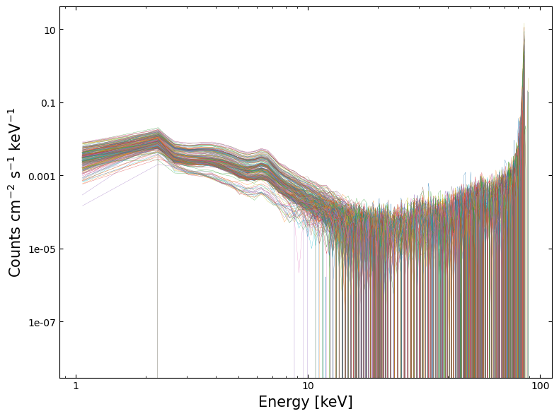
Visualizing the spectra#
Using the data extracted in the last step, we can plot the spectra and fitted models using matplotlib.
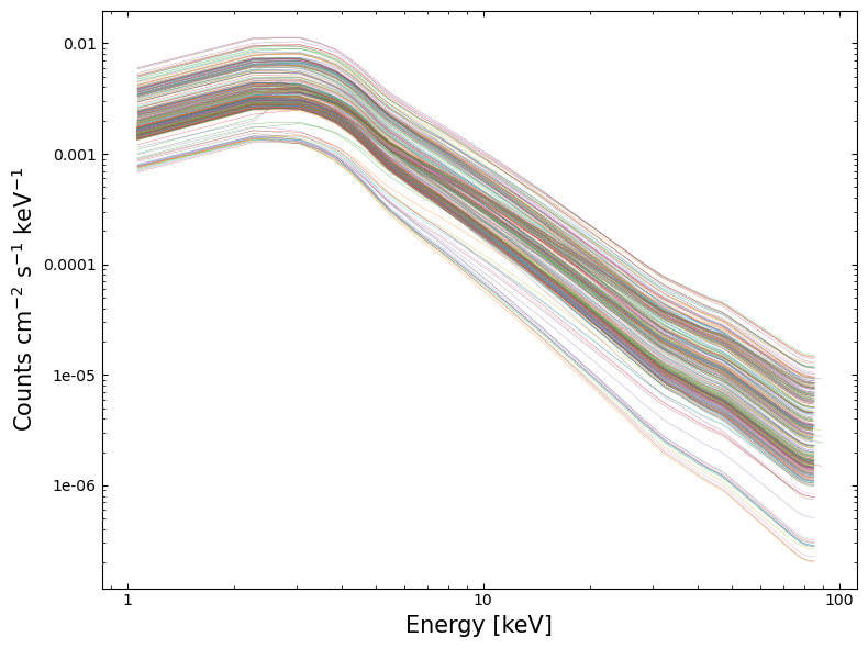
Visualizing the fitted models#
4. Exploring model fit results#
As we have fit models to all these spectra and retrieved the parameter’s values, we should take a look at them!
Exactly what you do at this point will depend entirely upon your science case and the type of object you’ve been analyzing. However, any analysis will benefit from an initial examination of the fitted parameter values (particularly if you have fit hundreds of spectra, as we have).
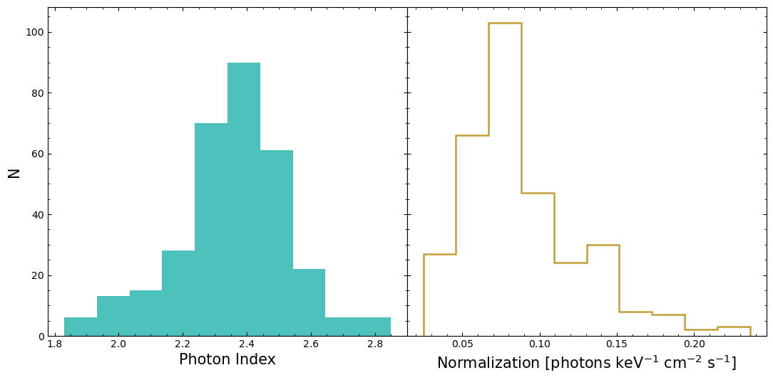
Fitted model parameter distributions#
This shows us what the distributions of the ‘Photon Index’ (related to the power-law slope) and the model normalization look like. We can see that the distributions are not particularly symmetric and Gaussian-looking.
Do model parameters vary with time?#
That might then make us wonder if the reason we’re seeing these non-Gaussian distributions is due to Eta Car’s X-ray emission varying with time over the course of RXTE’s campaign? Some kinds of X-ray sources are extremely variable, and we know that Eta Car’s X-ray emission is variable in other wavelengths.
As a quick check, we can retrieve the start time of each RXTE observation from the source spectra and then plot the model parameter values against the time of their observation. In this case, we extract the modified Julian date (MJD) reference time, the time system, and the start time (which is currently relative to the reference time). Combining this information lets us convert the start time into a datetime object.
obs_start = []

for loc_sp in src_sp_files:
    with fits.open(os.path.join(spec_file_path, loc_sp)) as speco:
        cur_ref = Time(
            speco[0].header["MJDREFI"] + speco[0].header["MJDREFF"], format="mjd"
        )
        cur_tstart = Quantity(speco[0].header["TSTART"], "s")
        start_dt = (
            cur_ref
            + TimeDelta(
                cur_tstart, format="sec", scale=speco[0].header["TIMESYS"].lower()
            )
        ).to_datetime()
        obs_start.append(start_dt)
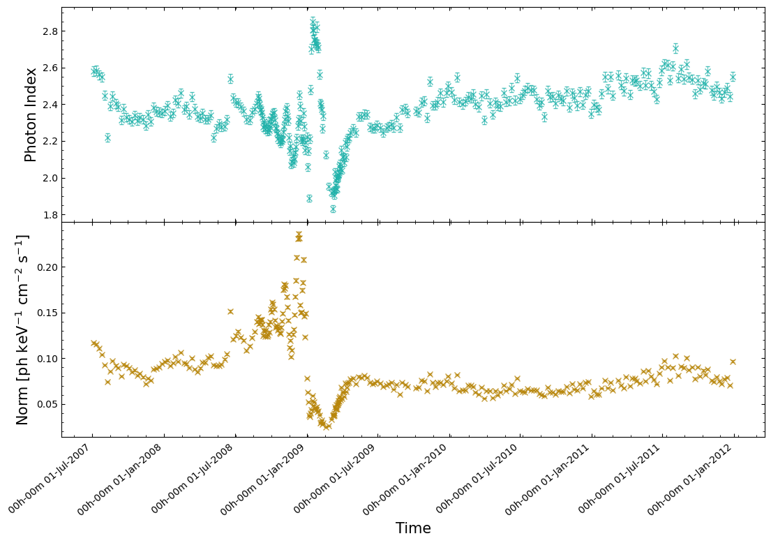
Now we actually plot the Photon Index and Normalization values against the start times, and we can see an extremely strong indication of time varying X-ray emission from Eta Car:
5. Applying simple unsupervised machine learning to the spectra#
From our previous analysis, fitting a simple power-law model to the spectra and plotting the parameters against the time of their observation, we can see that some quite interesting spectral changes occur over the course of RXTE’s survey visits to Eta Car.
We might now want to know whether we can identify those same behaviors in a model independent way, to ensure that it isn’t just a strange emergent property of spectral model choice.
Additionally, if the spectral changes we observed through the fitted model parameters are representative of real behavior, then are we seeing a single transient event where the emission returns to ‘normal’ after the most significant changes, or is it entering a new ‘phase’ of its emission life cycle?
We are going to use some very simple machine learning techniques to explore these questions by:
Reducing the spectra (with around one hundred energy bins and corresponding spectral values) to two dimensions.
Using a clustering technique to group similar spectra together.
Examining which spectra have been found to be the most similar.
Preparing#
Simply shoving the RXTE spectra that we already loaded in through some machine learning techniques is not likely to produce useful results.
Machine learning techniques that reduce dataset dimensionality often benefit from re-scaling the datasets so that all features (the spectral value for a particular energy bin, in this case) exist within the same general range (-1 to 1, for example). This is because the distance between points is often used as some form of metric in these techniques, and we wish to give every feature the same weight in those calculations.
It will hopefully mean that, for instance, the overall normalization isn’t the one dominant factor in grouping the spectra together, and instead other features (particularly the shape of a spectrum) will be given weight as well.
Interpolating the spectra onto a common energy grid#
Our first step is to place all the spectra onto a common energy grid. Due to changing calibration and instrument response, we cannot guarantee that the energy bins of all our spectra are identical.
Looking at the first few energy bins of two different spectra, as an example:
print(spec_plot_data[0][0][:5])
print(spec_plot_data[40][0][:5])
[1.0708092413842678, 2.2686474323272705, 2.669748067855835, 3.0714478492736816, 3.473743438720703]
[1.0690011642873287, 2.2649662494659424, 2.6654340028762817, 3.0664981603622437, 3.4681555032730103]
The quickest and easiest way to deal with this is to define a common energy grid and then interpolate all of our spectra onto it.
We choose to begin the grid at 2 keV to avoid low-resolution noise at lower energies, a limitation of RXTE-PCA data, and to stop it at 12 keV due to a noticeable lack of emission from Eta Car above that energy. The grid will have a resolution of 0.1 keV.
# Defining the specified energy grid
interp_en_vals = np.arange(2.0, 12.0, 0.1)

# Iterate through all loaded RXTE-PCA spectra
interp_spec_vals = []
for spec_info in spec_plot_data:
    # This runs the interpolation, using the values we extracted from PyXspec earlier.
    #  spec_info[0] are the energy values, and spec_info[2] the spectral values
    interp_spec_vals.append(np.interp(interp_en_vals, spec_info[0], spec_info[2]))

# Make the interpolated spectra into a numpy array
interp_spec_vals = np.array(interp_spec_vals)
Scaling and normalizing the spectra#
As we’ve already mentioned, the machine learning techniques we’re going to use will work best if the input data
are scaled. This StandardScaler class will move the mean of each feature (spectral value in an energy bin) to zero
and scale it unit variance.
scaled_interp_spec_vals = StandardScaler().fit_transform(interp_spec_vals)
Examining the scaled and normalized spectra#
To demonstrate the changes we’ve made to our dataset, we’ll visualize both the interpolated and the scaled-interpolated spectra:
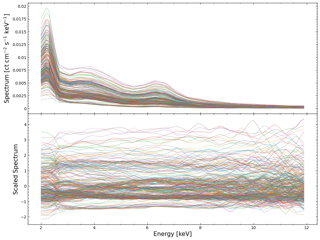
Reducing the dimensionality of the scaled spectral dataset#
At this point, we could try to find similar spectra by applying a clustering technique directly to the scaled dataset we just created. However, it has been well demonstrated that finding similar data points (clustering them together, in other words) is very difficult in high-dimensional data.
This is a result of something called “the curse of dimensionality” (see, Karanam, Shashmi; 2021, for an overview), a common problem in machine learning and data science.
One of the ways to combat this issue is to try and reduce the dimensionality of the dataset. The hope is that the data point that represents a spectrum (in N dimensions, where N is the number of energy bins in our interpolated spectrum) can be projected/reduced to a much smaller number of dimensions without losing the information that will help us group the different spectra.
We’re going to try three common dimensionality reduction techniques:
Principal Component Analysis (PCA)
T-distributed Stochastic Neighbor Embedding (t-SNE)
Uniform Manifold Approximation and Projection (UMAP)
An article by Varma, Aastha (2024) provides simple summaries of these three techniques and when they can be used. We encourage you to identify resources that explain whatever dimensionality reduction technique you may end up using, as it is all too easy to treat these techniques as black boxes.
Principal Component Analysis (PCA)#
PCA is arguably the simplest of the dimensionality reduction techniques that we’re trying out in this demonstration. The technique works by projecting the high-dimensionality data into a lower-dimension parameter space (two dimensions, in this case) whilst maximizing the variance of the projected data.
PCA is best suited to linearly separable data, but isn’t particularly suitable for non-linear relationships.
pca = PCA(n_components=2)

scaled_specs_pca = pca.fit_transform(scaled_interp_spec_vals)
T-distributed Stochastic Neighbor Embedding (t-SNE)#
Unlike PCA, t-SNE is suited to non-linearly separable data, though it is also much more computationally expensive. This technique works by comparing two distributions:
Pairwise similarities (defined by some distance metric) of the data points in the original high-dimensional data.
The equivalent similarities but in the projected two-dimensional space.
The goal is to minimize the divergence between the two distributions and effectively try to represent the same spacings between data points in N-dimensions in a two-dimensional space.
tsne = TSNE(n_components=2)
scaled_specs_tsne = tsne.fit_transform(scaled_interp_spec_vals)
Uniform Manifold Approximation and Projection (UMAP)#
Finally, the UMAP technique is also well suited to non-linearly separable data. It also does well at preserving and representing local and global structures from the original N-dimensional data in the output two-dimensional (in our case) space.
UMAP in particular is mathematically complex (compared to the other two techniques we’re using) - a full explanation by the UMAP Contributors is included in the documentation.
The original paper describing UMAP (McInnes et al. 2018) may also be useful.
um = UMAP(random_state=1, n_jobs=1)
scaled_specs_umap = um.fit_transform(scaled_interp_spec_vals)
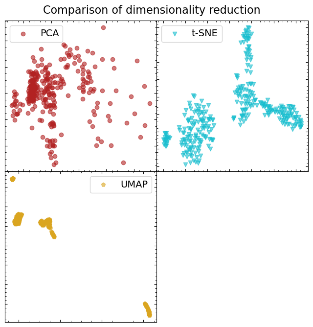
Comparing the results of the different dimensionality reduction methods#
In each case, we reduced the scaled spectral dataset to two dimensions, so it is easy to visualize how each technique has behaved. We’re going to visually assess the separability of data point groups (we are starting with the assumption that there will be some distinct groupings of spectra).
Just from a quick look, it is fairly obvious that UMAP has done the best job of forming distinct, separable, groupings of spectra. That doesn’t necessarily mean that those spectra are somehow physically linked, but it does seem like it will be the best dataset to run our clustering algorithm on.
Automated clustering of like spectra with Density-Based Spatial Clustering of Applications with Noise (DBSCAN)#
There are a litany of clustering algorithms implemented in scikit-learn, all with different characteristics, strengths, and weaknesses. The scikit-learn website provides an interesting comparison (Scikit-learn Contributors) of their performance on different toy datasets, which gives an idea of what sorts of features can be separated with each approach.
Some algorithms require that you specify the number of clusters you want to find, which is not particularly easy to do while doing this sort of exploratory data analysis. As such, we’re going to use ‘DBSCAN’, which identifies dense cores of data points and expands clusters from them. You should read about a variety of clustering techniques and how they work before deciding on one to use for your own scientific work.
dbs = DBSCAN(eps=0.6, min_samples=2)
clusters = dbs.fit(scaled_specs_umap)

# The labels of the point clusters
clust_labels = np.unique(clusters.labels_)
clust_labels
array([0, 1, 2, 3, 4, 5, 6])
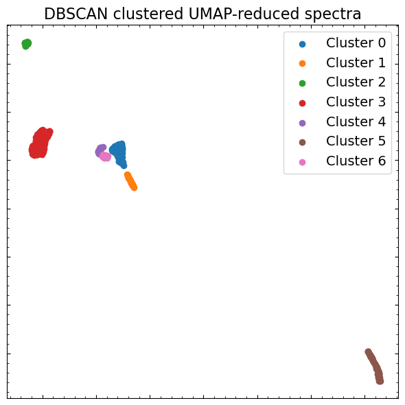
We will once again visualize the UMAP-reduced spectral dataset, but this time we’ll color each data point by the cluster that DBSCAN says it belongs to. That will give us a good idea of how well the algorithm has performed:
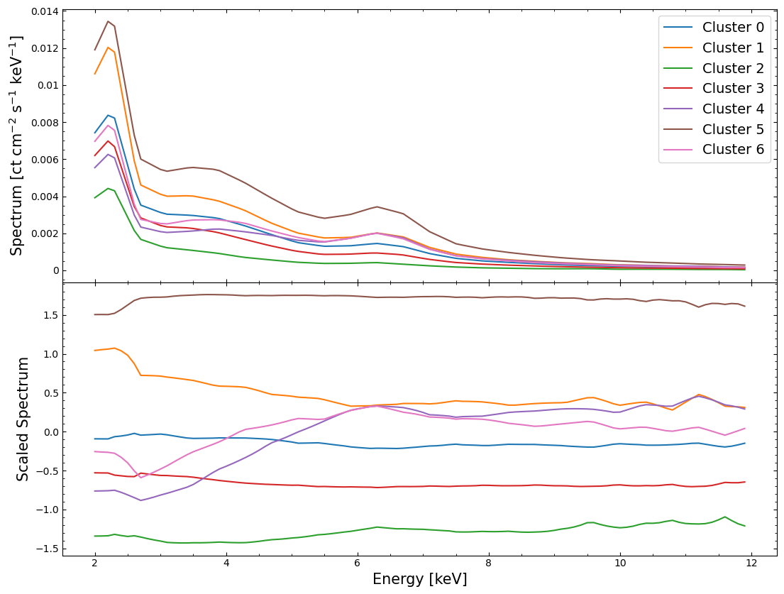
Exploring the results of spectral clustering#
Now that we think we’ve identified distinct groupings of spectra that are similar (in the two-dimensional space produced by UMAP at least), we can look to see whether they look distinctly different in their original high-dimensional parameter space!
Here we examine both unscaled and scaled versions of the interpolated spectra, but rather than coloring every individual spectrum by the cluster that it belongs to, we instead plot the mean spectrum of each cluster.
This approach makes it much easier to interpret the figures, and we can see straight away that most of the mean spectra of the clusters are quite distinct from one another:
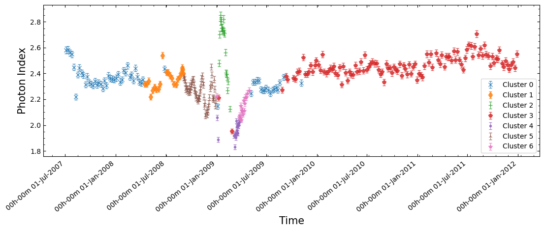
Having done all of this, we can return to the original goal of this section and look to see whether the significant time-dependent behaviors of our fitted model parameters are also identified through this model-independent approach. Additionally, if they are identified this way, are the spectra before and after the most significant changes different, or did the emission return to ‘normal’ after the disruption?
We plot the same figure of power-law photon index versus time that we did earlier, but now we can color the data points by which point cluster their spectrum is associated with.
From this plot it seems like the significant fluctuations of photon index with time are not an emergent property of our model choice, and instead represent real differences in the RXTE-PCA spectra of Eta Car at different observation times!
About this notebook#
Author: Tess Jaffe, HEASARC Chief Archive Scientist.
Author: David J Turner, HEASARC Staff Scientist.
Updated On: 2026-01-19
Additional Resources#
Support: HEASARC RXTE Helpdesk
Documents:
Acknowledgements#
References#
Varma, Aastha (2024) - ‘Dimensionality Reduction: PCA, t-SNE, and UMAP’ [ACCESSED 19-JAN-2026]