Getting started with Swift-XRT#
Learning Goals#
This tutorial will teach you how to:
Identify and download Swift observations of a particular source (we use the recurrent nova T Pyx to demonstrate).
Prepare Swift X-ray Telescope (XRT) data for scientific use, producing ‘level 2’ cleaned event lists.
Generate Swift-XRT data products, including:
Exposure maps
Images
Spectra
Light curves
Perform a simple spectral analysis.
Introduction#
This notebook is intended to introduce you to the use of data taken by the Swift mission’s X-ray Telescope (XRT) instrument and to provide a template or starting point for performing your own analysis.
Swift is a high-energy mission designed for extremely fast reaction times to transient high-energy phenomena, particularly Gamma-ray Bursts (GRBs). The Burst Alert Telescope (BAT) instrument has a very large field-of-view (FoV; ~2 steradians), and when it detects a GRB, it will typically start to slew in ~10 seconds. That means that Swift’s other two instruments, XRT and the Ultra-violet Optical Telescope (UVOT), both with much smaller FoVs, can be brought to bear on the GRB quickly.
Though designed with GRBs in mind, Swift’s quick reaction times and wide wavelength coverage make it useful for many other transient phenomena, ‘recurrent novae’ for instance.
Novae are multi-wavelength transients powered by a thermonuclear runaway on the surface of an accreting white dwarf. At early times during the eruption (the first month or two), the X-ray emission is relatively hard and produced thermally by shock-heated gas inside the ejecta. This hard X-ray emission can be faint and is not always detectable with Swift-XRT (or any other X-ray telescope for that matter). As the nova evolves, the ejecta thins out, and we get a view of the white dwarf’s surface, where there is residual nuclear burning. This nuclear burning emits predominantly in the far UV/soft X-ray bands and produces a bright super-soft X-ray transient, often modeled as a blackbody, sometimes with some residual hard X-rays from shock-heated gas remaining. This component is usually visible with Swift-XRT for reasonably nearby Galactic novae like T Pyx, and the XRT count rates can vary anywhere from under 0.01 ct s\(^{-1}\) to ~300 ct s\(^{-1}\).
Using a recurrent nova as an example, we will take you, from first principles, through the process of identifying Swift-XRT observations of an object of interest, downloading and processing the data, generating common X-ray data products, and performing a simple spectral analysis. Work undertaken by Chomiuk et al. (2014) inspired many of the demonstrations in this notebook.
We will use the Python interface to HEASoft (HEASoftPy) throughout this notebook.
Inputs#
The name of the source (T Pyx) we want to investigate.
Discovery time of T Pyx’s sixth historical outburst (55665 MJD).
Outputs#
X-ray data products (images, exposure maps, spectra, light curves, etc.) for our selection of Swift observations.
Visualizations of Swift-XRT images, centered on T Pyx.
Visualizations of T Pyx Swift-XRT spectra, as well as fitted spectral models.
Runtime#
As of 31st October 2025, this notebook takes ~16 minutes to run to completion on Fornax using the ‘Default Astrophysics’ image and the ‘medium’ server with 16GB RAM/ 4 cores.
Imports#
import contextlib
import glob
import multiprocessing as mp
import os
from copy import deepcopy
from typing import Tuple, Union
from warnings import warn

import heasoftpy as hsp
import matplotlib.pyplot as plt
import numpy as np
import xspec as xs
from astropy.coordinates import SkyCoord
from astropy.time import Time
from astropy.units import Quantity
from astropy.visualization import PowerStretch
from astroquery.heasarc import Heasarc
from IPython.display import Markdown, display
from matplotlib.ticker import FuncFormatter
from tqdm import tqdm
from xga.imagetools.misc import pix_deg_scale
from xga.products import EventList, Image
/opt/envs/heasoft/lib/python3.12/site-packages/xga/utils.py:39: DeprecationWarning: The XGA 'find_all_wcs' function should be imported from imagetools.misc, in the future it will be removed from utils.
  warn(message, DeprecationWarning)
/opt/envs/heasoft/lib/python3.12/site-packages/xga/utils.py:619: UserWarning: SAS_DIR environment variable is not set, unable to verify SAS is present on system, as such all functions in xga.sas will not work.
  warn("SAS_DIR environment variable is not set, unable to verify SAS is present on system, as such "
Global Setup#
Functions#
Constants#
Configuration#
1. Finding and downloading Swift observations of T Pyx#
Our first task is to determine which Swift observations are relevant to the source that we are interested in, the recurrent nova T Pyx.
We are going in with the knowledge that T Pyx has been observed by Swift, but of course there is no guarantee that your source of interest has been, so this is an important exploratory step.
Identifying the Swift observation summary table#
HEASARC maintains tables that contain information about every observation taken by each of the missions in its archive. We will use Swift’s table to find observations that should be relevant to our source.
The name of the Swift observation summary table is ‘swiftmastr’, but as you may not know that a priori, we demonstrate how to identify the correct table for a given mission.
Using the AstroQuery Python module (specifically this Heasarc object), we list all catalogs that are a) related to Swift, and b) are flagged as ‘master’ (meaning the summary table of observations). This should only return one catalog for any mission you pass to ‘keywords’:
catalog_name = Heasarc.list_catalogs(master=True, keywords="swift")[0]["name"]
catalog_name
np.str_('swiftmastr')
What are the coordinates of the target?#
To search for relevant observations, we have to know the coordinates of our source. The astropy module allows us to look up a source name in CDS’ Sesame name resolver and retrieve its coordinates.
Hint
You could also set up a SkyCoord object directly, if you already know the coordinates.
src_coord = SkyCoord.from_name(SRC_NAME)
# This will be useful later on in the notebook, for functions that take
#  coordinates as an astropy Quantity.
src_coord_quant = Quantity([src_coord.ra, src_coord.dec])
src_coord
<SkyCoord (ICRS): (ra, dec) in deg
    (136.1729423, -32.37986193)>
Searching for Swift observations of T Pyx#
Now that we know which catalog to search, and the coordinates of our source, we use AstroQuery to retrieve those lines of the summary table that are within some radius of the source coordinate.
Each mission’s observation summary table has its own default search radius, normally based on the size of the telescope’s FoV.
Defining a default radius for missions that have multiple instruments with very different FoVs (like Swift) can be challenging, so it is always a good idea to check what the default value is:
Heasarc.get_default_radius(catalog_name)
That default radius suits our purposes, but if it hadn’t, then we could have overridden
it by passing a different value to the radius keyword argument.
We run the query and receive a subset of the master table containing information about the relevant observations. The returned table is then sorted by ascending start time, which will make our lives easier later in the notebook when we examine how T Pyx has changed over time.
swift_obs = Heasarc.query_region(src_coord, catalog_name)

# We sort by start time, so the table is in order of ascending start
swift_obs.sort("start_time", reverse=False)

swift_obs
| name | obsid | ra | dec | start_time | processing_date | xrt_exposure | uvot_exposure | bat_exposure | archive_date | __row |
|---|---|---|---|---|---|---|---|---|---|---|
| deg | deg | d | d | s | s | s | d | |||
| object | object | float64 | float64 | float64 | float64 | float64 | float64 | float64 | int32 | object |
| TPyx | 00031968001 | 136.15226 | -32.37080 | 55665.587349537 | 57643.0 | 2597.30600 | 0.00000 | 2616.00000 | 55676 | 130422 |
| TPyx | 00031968002 | 136.14748 | -32.36878 | 55666.7291666667 | 57643.0 | 1201.15300 | 0.00000 | 1218.00000 | 55677 | 130432 |
| TPyx | 00031968003 | 136.14294 | -32.36096 | 55667.7388888889 | 57829.0 | 1474.82100 | 0.00000 | 1492.00000 | 55678 | 130520 |
| TPyx | 00031968004 | 136.09599 | -32.36940 | 55668.7347222222 | 57643.0 | 1060.73900 | 0.00000 | 1077.00000 | 55679 | 130428 |
| TPyx | 00031968005 | 136.14678 | -32.36484 | 55669.7458333333 | 57829.0 | 1438.27800 | 0.00000 | 1456.00000 | 55680 | 130496 |
| TPyx | 00031968006 | 136.14076 | -32.37281 | 55670.6833333333 | 57829.0 | 2404.49000 | 0.00000 | 2438.00000 | 55681 | 130414 |
| TPyx | 00031968007 | 136.09743 | -32.37885 | 55671.4797106481 | 57644.0 | 1011.84600 | 0.00000 | 1159.00000 | 55682 | 130333 |
| TPyx | 00031968008 | 136.16624 | -32.38262 | 55672.6215162037 | 57644.0 | 252.47500 | 253.30500 | 600.00000 | 55683 | 130266 |
| TPyx | 00031968009 | 136.17396 | -32.38026 | 55672.6243055556 | 57644.0 | 2174.58900 | 2133.33400 | 1908.00000 | 55683 | 130276 |
| ... | ... | ... | ... | ... | ... | ... | ... | ... | ... | ... |
| TPyx | 00031968156 | 136.15184 | -32.35719 | 55990.506400463 | 57859.0 | 1837.08200 | 1799.89800 | 1850.00000 | 56001 | 130627 |
| TPyx | 00031968157 | 136.14956 | -32.36261 | 55993.0965277778 | 57859.0 | 2253.56100 | 2197.52200 | 2277.00000 | 56004 | 130510 |
| TPyx | 00031968158 | 136.13731 | -32.35809 | 55994.1659606481 | 57859.0 | 3045.52100 | 2972.94200 | 3074.00000 | 56005 | 130620 |
| TPyx | 00031968159 | 136.16011 | -32.40473 | 56002.6583333333 | 57859.0 | 77.31700 | 77.14200 | 84.00000 | 56013 | 130100 |
| TPyx | 00031968160 | 136.10975 | -32.35739 | 56010.2152777778 | 57859.0 | 3194.91300 | 3153.44100 | 3209.00000 | 56021 | 130626 |
| TPyx | 00031968161 | 136.12736 | -32.40198 | 56018.9118055556 | 57865.0 | 2820.94800 | 2780.90400 | 2836.00000 | 56029 | 130112 |
| TPyx | 00031968162 | 136.14563 | -32.36482 | 56026.1201388889 | 57865.0 | 3158.35600 | 3042.03300 | 3195.00000 | 56037 | 130497 |
| TPyx | 00031968163 | 136.14416 | -32.36998 | 56034.3395833333 | 57865.0 | 2772.56300 | 2677.27100 | 2809.00000 | 56045 | 130426 |
| TPyx | 00031968164 | 136.15470 | -32.36690 | 56384.2117939815 | 58065.0 | 5183.62400 | 5146.10700 | 5204.00000 | 56395 | 130436 |
Cutting down the Swift observations for this tutorial#
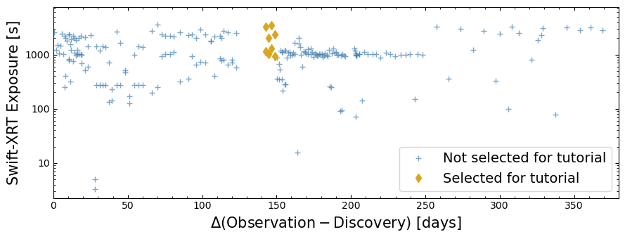
The table we just retrieved shows that T Pyx has been observed by Swift many times, but in order to shorten the run time of this demonstration, we’re going to select a subset of the available observations.
We select observations that were taken in a period of between 142 and 149 days after the discovery of T Pyx’s sixth outburst, a time in which it was particularly X-ray bright.
# Defining an Astropy Time object, to match the Time object we defined
#  to hold the discovery time, in the global setup section.
obs_times = Time(swift_obs["start_time"], format="mjd")

# Simply subtract the discovery time from the observation times to get the delta
obs_day_from_disc = (obs_times - DISC_TIME).to("day")

# Make a dictionary of that information with ObsIDs as keys, which will make
#  some plotting code neater later on in the notebook
obs_day_from_disc_dict = {
    oi: obs_day_from_disc[oi_ind] for oi_ind, oi in enumerate(swift_obs["obsid"])
}
Now we’ll apply the time window constraints by creating a boolean array that can be applied to the retrieved observation table as a mask:
sel_mask = (obs_day_from_disc > Quantity(142, "day")) & (
    obs_day_from_disc < Quantity(149, "day")
)
The mask is applied to the original table of relevant observations, and we also read out our selected ObsIDs into another variable, for later use:
cut_swift_obs = swift_obs[sel_mask]
rel_obsids = np.array(cut_swift_obs["obsid"])

cut_swift_obs
| name | obsid | ra | dec | start_time | processing_date | xrt_exposure | uvot_exposure | bat_exposure | archive_date | __row |
|---|---|---|---|---|---|---|---|---|---|---|
| deg | deg | d | d | s | s | s | d | |||
| object | object | float64 | float64 | float64 | float64 | float64 | float64 | float64 | int32 | object |
| TPyx | 00031968059 | 136.20108 | -32.38330 | 55807.7458333333 | 57660.0 | 1132.55700 | 1070.21100 | 1500.00000 | 55818 | 130265 |
| TPyx | 00032089001 | 136.04758 | -32.31409 | 55807.7513888889 | 57660.0 | 3269.49300 | 3078.11900 | 3019.00000 | 55818 | 130458 |
| TPyx | 00031968060 | 136.15998 | -32.38590 | 55809.6173611111 | 57660.0 | 1020.44500 | 960.60400 | 1294.00000 | 55820 | 130255 |
| TPyx | 00032089002 | 136.04691 | -32.31299 | 55809.6229050926 | 57660.0 | 2017.86600 | 1858.87000 | 1839.00000 | 55820 | 130463 |
| TPyx | 00031968061 | 136.22223 | -32.37604 | 55811.4979166667 | 57660.0 | 1294.37800 | 1238.56600 | 1800.00000 | 55822 | 130349 |
| TPyx | 00032089004 | 136.04593 | -32.31546 | 55811.5048611111 | 57660.0 | 3414.31100 | 3268.16000 | 2993.00000 | 55822 | 130454 |
| TPyx | 00031968062 | 136.16252 | -32.38602 | 55813.8319444444 | 57660.0 | 937.09900 | 898.66900 | 1200.00000 | 55824 | 130253 |
| TPyx | 00032089005 | 136.05578 | -32.31443 | 55813.8388888889 | 57660.0 | 2326.41500 | 2231.70600 | 2150.00000 | 55824 | 130457 |
To put them into context, we plot the selected time-window-limited subset of relevant observations, and all the other relevant observations, on a figure showing the nominal Swift-XRT exposure time against the time since the discovery of T Pyx’s sixth outburst.
Downloading the selected Swift observations#
We’ve settled on the observations that we’re going to use during the course of this
tutorial and now need to actually download them. The easiest way to do this is to
use another feature of the AstroQuery Heasarc object, which will take the table
of chosen observations and identify ‘data links’ for each of them.
The data links describe exactly where the particular data can be downloaded from - for HEASARC data the most relevant places would be the HEASARC FTP server and the HEASARC Amazon Web Services (AWS) S3 bucket.
data_links = Heasarc.locate_data(cut_swift_obs)
data_links
| ID | access_url | sciserver | aws | content_length | error_message |
|---|---|---|---|---|---|
| byte | |||||
| object | object | str40 | str53 | int64 | object |
| ivo://nasa.heasarc/swiftmastr?130253 | https://heasarc.gsfc.nasa.gov/FTP/swift/data/obs/2011_09//00031968062/ | /FTP/swift/data/obs/2011_09/00031968062/ | s3://nasa-heasarc/swift/data/obs/2011_09/00031968062/ | 9989972 | |
| ivo://nasa.heasarc/swiftmastr?130255 | https://heasarc.gsfc.nasa.gov/FTP/swift/data/obs/2011_09//00031968060/ | /FTP/swift/data/obs/2011_09/00031968060/ | s3://nasa-heasarc/swift/data/obs/2011_09/00031968060/ | 11146423 | |
| ivo://nasa.heasarc/swiftmastr?130265 | https://heasarc.gsfc.nasa.gov/FTP/swift/data/obs/2011_09//00031968059/ | /FTP/swift/data/obs/2011_09/00031968059/ | s3://nasa-heasarc/swift/data/obs/2011_09/00031968059/ | 16683297 | |
| ivo://nasa.heasarc/swiftmastr?130349 | https://heasarc.gsfc.nasa.gov/FTP/swift/data/obs/2011_09//00031968061/ | /FTP/swift/data/obs/2011_09/00031968061/ | s3://nasa-heasarc/swift/data/obs/2011_09/00031968061/ | 33950072 | |
| ivo://nasa.heasarc/swiftmastr?130454 | https://heasarc.gsfc.nasa.gov/FTP/swift/data/obs/2011_09//00032089004/ | /FTP/swift/data/obs/2011_09/00032089004/ | s3://nasa-heasarc/swift/data/obs/2011_09/00032089004/ | 134191346 | |
| ivo://nasa.heasarc/swiftmastr?130457 | https://heasarc.gsfc.nasa.gov/FTP/swift/data/obs/2011_09//00032089005/ | /FTP/swift/data/obs/2011_09/00032089005/ | s3://nasa-heasarc/swift/data/obs/2011_09/00032089005/ | 72037009 | |
| ivo://nasa.heasarc/swiftmastr?130458 | https://heasarc.gsfc.nasa.gov/FTP/swift/data/obs/2011_09//00032089001/ | /FTP/swift/data/obs/2011_09/00032089001/ | s3://nasa-heasarc/swift/data/obs/2011_09/00032089001/ | 134506155 | |
| ivo://nasa.heasarc/swiftmastr?130463 | https://heasarc.gsfc.nasa.gov/FTP/swift/data/obs/2011_09//00032089002/ | /FTP/swift/data/obs/2011_09/00032089002/ | s3://nasa-heasarc/swift/data/obs/2011_09/00032089002/ | 97760516 |
Passing the data links to the Heasarc.download_data function, and setting the
ROOT_DATA_DIR variable as the output directory, will download the Swift data to
the desired location.
This approach will download the entire data directory for a given Swift observation, which will include BAT and UVOT instrument files that are not relevant to this tutorial.
Heasarc.download_data(data_links, "aws", ROOT_DATA_DIR)
INFO: Downloading data AWS S3 ... [astroquery.heasarc.core]
INFO: Enabling anonymous cloud data access ... [astroquery.heasarc.core]
INFO: downloading s3://nasa-heasarc/swift/data/obs/2011_09/00031968062/ [astroquery.heasarc.core]
INFO: downloading s3://nasa-heasarc/swift/data/obs/2011_09/00031968060/ [astroquery.heasarc.core]
INFO: downloading s3://nasa-heasarc/swift/data/obs/2011_09/00031968059/ [astroquery.heasarc.core]
INFO: downloading s3://nasa-heasarc/swift/data/obs/2011_09/00031968061/ [astroquery.heasarc.core]
INFO: downloading s3://nasa-heasarc/swift/data/obs/2011_09/00032089004/ [astroquery.heasarc.core]
INFO: downloading s3://nasa-heasarc/swift/data/obs/2011_09/00032089005/ [astroquery.heasarc.core]
INFO: downloading s3://nasa-heasarc/swift/data/obs/2011_09/00032089001/ [astroquery.heasarc.core]
INFO: downloading s3://nasa-heasarc/swift/data/obs/2011_09/00032089002/ [astroquery.heasarc.core]
Note
We choose to download the data from the HEASARC AWS S3 bucket, but you could pass ‘heasarc’ to acquire data from the FTP server. Additionally, if you are working on SciServer, you may pass ‘sciserver’ to use the pre-mounted HEASARC dataset.
What do the downloaded data directories contain?#
glob.glob(os.path.join(ROOT_DATA_DIR, rel_obsids[0], "") + "*")
['/home/jovyan/projects/heasarc-tutorials/_data/Swift/00031968059/auxil',
 '/home/jovyan/projects/heasarc-tutorials/_data/Swift/00031968059/log',
 '/home/jovyan/projects/heasarc-tutorials/_data/Swift/00031968059/uvot',
 '/home/jovyan/projects/heasarc-tutorials/_data/Swift/00031968059/bat',
 '/home/jovyan/projects/heasarc-tutorials/_data/Swift/00031968059/xrt']
glob.glob(os.path.join(ROOT_DATA_DIR, rel_obsids[0], "xrt", "") + "**/*")
['/home/jovyan/projects/heasarc-tutorials/_data/Swift/00031968059/xrt/event/sw00031968059xwtw2st_cl.evt.gz',
 '/home/jovyan/projects/heasarc-tutorials/_data/Swift/00031968059/xrt/event/sw00031968059xpcw3po_cl.evt.gz',
 '/home/jovyan/projects/heasarc-tutorials/_data/Swift/00031968059/xrt/event/sw00031968059xwtw2st_uf.evt.gz',
 '/home/jovyan/projects/heasarc-tutorials/_data/Swift/00031968059/xrt/event/sw00031968059xwtw2sl_cl.evt.gz',
 '/home/jovyan/projects/heasarc-tutorials/_data/Swift/00031968059/xrt/event/sw00031968059xpcw3po_uf.evt.gz',
 '/home/jovyan/projects/heasarc-tutorials/_data/Swift/00031968059/xrt/event/sw00031968059xwtw2sl_ufre.evt.gz',
 '/home/jovyan/projects/heasarc-tutorials/_data/Swift/00031968059/xrt/event/sw00031968059xwtw2sl_uf.evt.gz',
 '/home/jovyan/projects/heasarc-tutorials/_data/Swift/00031968059/xrt/event/sw00031968059xwtw2st_ufre.evt.gz',
 '/home/jovyan/projects/heasarc-tutorials/_data/Swift/00031968059/xrt/products/sw00031968059x_skim.gif',
 '/home/jovyan/projects/heasarc-tutorials/_data/Swift/00031968059/xrt/products/sw00031968059xpc_sk.img.gz',
 '/home/jovyan/projects/heasarc-tutorials/_data/Swift/00031968059/xrt/products/sw00031968059xpc_ex.img.gz',
 '/home/jovyan/projects/heasarc-tutorials/_data/Swift/00031968059/xrt/hk/sw00031968059xen.hk.gz',
 '/home/jovyan/projects/heasarc-tutorials/_data/Swift/00031968059/xrt/hk/sw00031968059xtr.hk.gz',
 '/home/jovyan/projects/heasarc-tutorials/_data/Swift/00031968059/xrt/hk/sw00031968059xbf_rw.img.gz',
 '/home/jovyan/projects/heasarc-tutorials/_data/Swift/00031968059/xrt/hk/sw00031968059xhd.hk.gz']
2. Processing the Swift-XRT data#
Though the Swift observations directories we downloaded already contain cleaned XRT event lists and pre-generated images, it is generally recommended that you reprocess Swift data yourself.
Reprocessing ensures that the latest versions of the preparation tools have been applied to your data.
Running the Swift XRT pipeline#
The software required to reprocess Swift-XRT observations is made available as part of the HEASoft package. There are quite a few Swift-XRT specific HEASoft tools, many of which are used as part of data processing, but a convenient processing pipeline (xrtpipeline) means that we don’t have to call the steps individually.
The pipeline is made up of three steps, with the user able to choose which step they wish to start and stop at. Per the xrtpipeline documentation, the steps perform the following processing steps:
Stage 1:
Hot pixel identification for photon-counting mode data.
Bad pixel identification for photon-counting and windowed-timing mode data.
Corrects housekeeping exposure times (TIME and ENDTIME columns) for timing mode frames.
Transforms coordinates for photon-counting, windowed-timing, and imaging mode data files.
Bias subtraction for photon-counting and imaging mode data.
Calculation of photon arrival times, and event recognition for timing mode data.
Screening on event GTIs to erase piled-up frames and partially exposed events for photo-diode mode data.
Event grade assignment for photon-counting and timing mode data.
Calculation of the PI for photon-counting, windowed-timing, and photo-diode mode data.
Stage 2:
Screening of the calibrated events produced in Stage 1 by applying conditions on a set of parameters. The screening is performed using GTIs obtained by applying conditions to housekeeping parameters specific to the instrument, and on attitude and orbit related quantities, a screening for bad pixels, and a constraints on acceptable event grades.
Stage 3:
Generating products for scientific analysis using the ‘xrtproducts’ task.
The HEASoftPy Python package provides a convenient interface to all HEASoft tasks, and we will use it to run the Swift-XRT processing pipeline. Additionally, we take advantage of the fact that multicore CPUs are now essentially ubiquitous, and we can perform parallel runs of xrtpipeline on individual observations. This significantly reduces the time it takes to process all the observations.
Swift-XRT can be operated in different data modes, but for the purposes of this tutorial we will focus only on the ‘photon counting’ (PC) mode, where XRT records the position, energy, and arrival time of each event. From those data we can eventually make images, light curves, and spectra. Other modes are more specialized, and beyond the scope of this tutorial.
Likewise, Swift has different ‘observation modes’ (pointed, slew, and settling) - we are only going to process and use the pointed data.
We set up a multiprocessing pool, and use starmap to call the process_swift_xrt
function with a different set of arguments for each ObsID - if there are more
observations than there are cores available, then the pool will manage
the allocation of tasks to cores. The data and observation modes are set within
our wrapper function.
The process_swift_xrt function is defined in the ‘Global Setup’ section of this
notebook, as we do not wish to interrupt the flow of this demonstration - you should
examine it to see how we call the HEASoftPy xrtpipeline task.
Our wrapper function also includes some error handling, meaning that if the processing of an observation fails for some reason, we can identify that observation and remove it from the list of relevant observations.
with mp.Pool(NUM_CORES) as p:
    arg_combs = [[oi, os.path.join(OUT_PATH, oi), src_coord] for oi in rel_obsids]
    pipe_result = p.starmap(process_swift_xrt, arg_combs)

xrt_pipe_problem_ois = [all_out[0] for all_out in pipe_result if not all_out[2]]
rel_obsids = [oi for oi in rel_obsids if oi not in xrt_pipe_problem_ois]

xrt_pipe_problem_ois
/opt/envs/heasoft/lib/python3.12/multiprocessing/popen_fork.py:66: DeprecationWarning: This process (pid=808) is multi-threaded, use of fork() may lead to deadlocks in the child.
  self.pid = os.fork()
[]
Warning
In this demonstration we set xrtpipeline to exit at stage 2, which is before the generation of X-ray data products. That is because we will run the xrtproducts task ourselves to give us more control over the outputs.
3. Generating Swift-XRT data products#
As we chose to stop the Swift-XRT processing pipeline at the second stage, we must now generate the X-ray data products that we want. Our primary reason for stopping the pipeline before this step is that we want to specify source and background regions ourselves, using region files.
We will create the images, light curves, spectra, and supporting files that we want using the HEASoftPy interface to the xrtproducts task, but will also use other HEASoft tools to generate Swift-XRT exposure maps, and to group the spectra.
Preparing for product generation#
It is useful at this stage to set up a variable to define the path to the clean event lists we output in the previous section. As we did not pass xrtpipeline arguments that modify the name of the event lists, they will have the default structure.
evt_path_temp = os.path.join(OUT_PATH, "{oi}/sw{oi}xpcw3po_cl.evt")
Now we create basic region files that define where the source and background spectra should be extracted from. In this case the source region is a circle, centered on the source coordinates, with a 180” radius, and the background region is an annulus around that source region, with a 240” radius and a 390” radius.
You might well wish to define more complex regions, particularly if there are bright sources close to the source you wish to analyze, and you would like to exclude them.
src_pos = src_coord.to_string("hmsdms", sep=":").replace(" ", ", ")

src_reg_path = os.path.join(OUT_PATH, "src.reg")

src_region = f'circle({src_pos}, 180")'
with open(src_reg_path, "w") as fp:
    fp.write("fk5\n")
    fp.write(src_region)

bck_reg_path = os.path.join(OUT_PATH, "bck.reg")

bgd_region = f'annulus({src_pos}, 240", 390")'
with open(bck_reg_path, "w") as fp:
    fp.write("fk5\n")
    fp.write(bgd_region)
Generating exposure maps#
The portion of xrtproducts that generates an ARF to accompany the source spectrum can use an exposure map to weight the PSF corrections applied to each portion of the extraction region. As the product generation pipeline does not create its own exposure maps, we will use the HEASoft xrtexpomap tool to make them here.
Some extra files are required by xrtexpomap, particularly the attitude file (which records the spacecraft attitude information throughout the observation) and the XRT housekeeping file (which contains detailed information about the state of the instrument).
Warning
Swift observation directories contain multiple attitude files, created in different ways. For some Swift processing tasks it is essential that the same attitude file used to create the event list is used - see this resource for more information. The header of the EVENTS table in the event file can identify the correct attitude file.
# We need to determine exactly which attitude file to use for each observation
att_files = {}
for oi in rel_obsids:
    cur_evts = EventList(evt_path_temp.format(oi=oi))
    att_ident = cur_evts.event_header["ATTFLAG"]
    if att_ident == "100":
        att_temp = "sw{oi}sat.fits.gz"
    elif att_ident == "110":
        att_temp = "sw{oi}pat.fits.gz"
    elif att_ident in ["111", "101"]:
        att_temp = "sw{oi}uat.fits.gz"

    att_files[oi] = os.path.join(ROOT_DATA_DIR, "{oi}/auxil", att_temp).format(oi=oi)

hd_file_temp = os.path.join(ROOT_DATA_DIR, "{oi}/xrt/hk/sw{oi}xhd.hk.gz")
We will once again run the XRT HEASoft tasks for our observations in parallel so that we can generate multiple exposure maps at once and speed up this notebook. Just like when we ran the xrtpipeline, here we have defined a wrapper function for the HEASoftPy interface to xrtexpomap, which can be found in the ‘Global Setup’ section of this notebook.
with mp.Pool(NUM_CORES) as p:
    arg_combs = [
        [
            evt_path_temp.format(oi=oi),
            os.path.join(OUT_PATH, oi),
            att_files[oi],
            hd_file_temp.format(oi=oi),
        ]
        for oi in rel_obsids
    ]

    exp_result = p.starmap(gen_xrt_expmap, arg_combs)
Generating light curves, images, and spectra#
We are finally ready to create light curves, images, and spectra from our Swift-XRT observations of T Pyx! The same multiprocessing setup used for xrtpipeline and xrtexpomap is implemented here, with a wrapper function defined in the ‘Global Setup’ section of this notebook.
Setting up a variable that defines the path to the exposure maps that we just generated, as we need to pass them to the xrtproducts task:
exp_map_temp = os.path.join(OUT_PATH, "{oi}/sw{oi}xpcw3po_ex.img")
Now we run the xrtproducts task, again parallelizing so that products for different observations are produced simultaneously. This tool will always produce full-FoV images in the 0.5-10.0 keV energy band, with a pixel size of 2.36”.
Whilst you cannot control the image energy band, you can specify PI channel limits for
light curves, using the pilow (default is 30) and pihigh (default is 1000)
arguments. For Swift-XRT (remember that different telescopes/instruments have
different channel-to-energy mappings) that corresponds to 0.3-10.0 keV. We
decide (somewhat arbitrarily) to generate light curves within the 0.5-2.5 keV energy
band.
lc_lo_en = (Quantity(0.5, "keV") / EV_PER_CHAN).to("chan")
lc_hi_en = (Quantity(2.5, "keV") / EV_PER_CHAN).to("chan")

with mp.Pool(NUM_CORES) as p:

    arg_combs = [
        [
            evt_path_temp.format(oi=oi),
            os.path.join(OUT_PATH, oi),
            src_reg_path,
            bck_reg_path,
            exp_map_temp.format(oi=oi),
            att_files[oi],
            hd_file_temp.format(oi=oi),
        ]
        for oi in rel_obsids
    ]

    prod_result = p.starmap(gen_xrt_im_spec, arg_combs)
Grouping the spectra#
Finally, we will group the spectra we just generated. Grouping essentially combines
spectral channels until some minimum quality threshold is reached; in this case a
minimum of one count per grouped channel. We use the HEASoft ftgrouppha tool to do
this, once again through HEASoftPy.
The reason we’re doing this is that the Cash statistic, which is very commonly used for statistical checks during X-ray spectral fitting, requires at least one count per grouped channel (or bin) to be valid. The Cash statistic is well suited to X-ray analysis, as more often than not, our data are quite Poissonian.
Once again we create variables that define the paths to relevant data products:
sp_temp = os.path.join(OUT_PATH, "{oi}/sw{oi}xpcw3posr.pha")
bsp_temp = os.path.join(OUT_PATH, "{oi}/sw{oi}xpcw3pobkg.pha")

grp_sp_temp = os.path.join(OUT_PATH, "{oi}/sw{oi}xpcw3posr_grp.pha")
Now we run the grouping tool - though this time we do not parallelize the task, as the grouping process is very fast, and we wish to demonstrate how you use a HEASoftPy function directly. Though remember to look at the Global Setup section of this notebook to see how we call HEASoftPy tools in the wrapper functions used to parallelize those tasks.
If you are dealing with significantly more observations than we use for this demonstration, we do recommend that you parallelize this grouping step as we have the other processing steps in this notebook.
for oi in rel_obsids:
    sp_path = sp_temp.format(oi=oi)
    bsp_path = bsp_temp.format(oi=oi)

    hsp.ftgrouppha(
        infile=sp_path,
        outfile=grp_sp_temp.format(oi=oi),
        grouptype="min",
        groupscale=1,
    )
Hint
Though we used a minimum count per grouped channel metric, ftgrouppha supports various other ways of binning a spectrum; e.g. uniform bin size, minimum signal-to-noise, and other ‘optimised’ binning algorithms (see the ftgrouppha help page for more information).
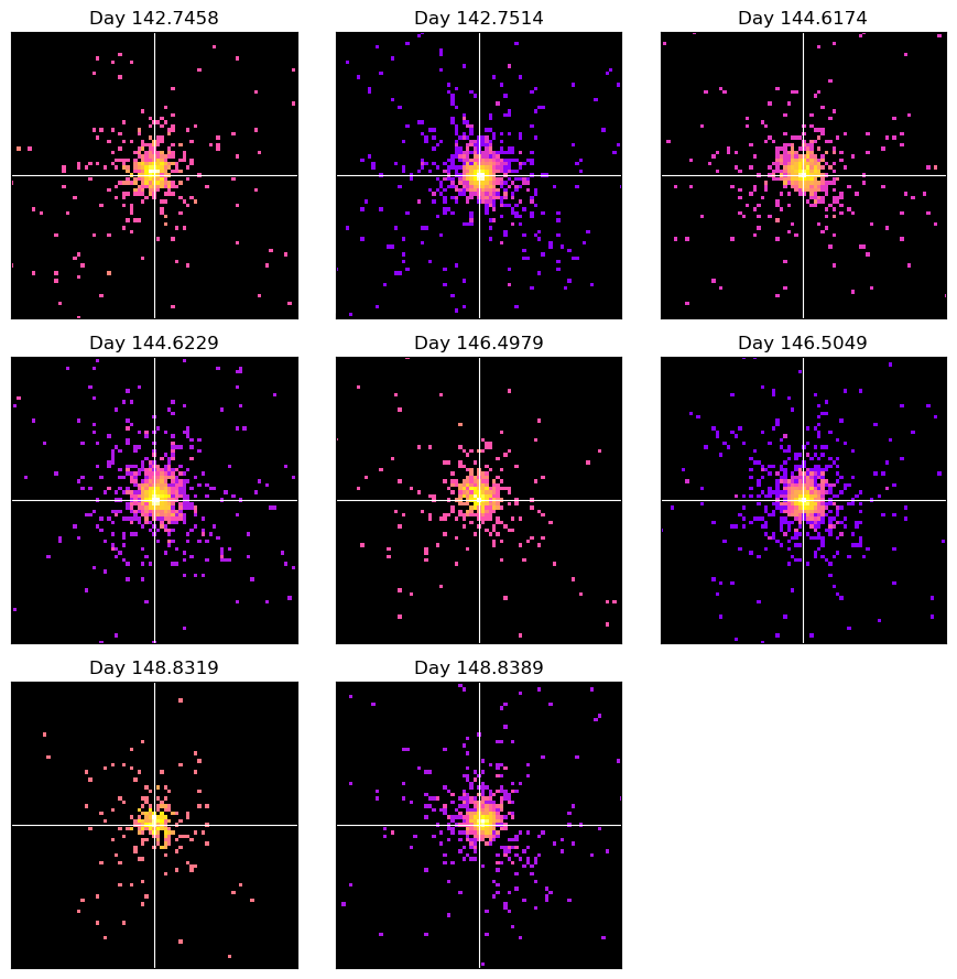
4. Examining the new Swift-XRT images#
When doing any sort of archival X-ray analysis (or indeed any kind of astrophysical work), we think it is important that you visually examine your data products. This serves both as a simple validity check and as a first chance to identify any interesting features in your data.
im_temp = os.path.join(OUT_PATH, "{oi}/sw{oi}xpcw3po_sk.img")
Here we create a simple figure with a separate panel for each Swift-XRT image we generated, making it easy to examine them all at once. In Section 1 we ordered the table of observations relevant to T Pyx by start time and placed the relevant ObsIDs into an array. We can now loop through that array and be assured that the images we plot will be in order of their observation’s start time.
To make the process a little easier, we make use of a Python module called
X-ray: Generate and Analyse (XGA); amongst other things, it implements Python classes
designed to make interacting with X-ray data products much easier. In this case we
will make use of a convenience function of the Image class that produces a
visualization of the data.
First, we load all our Swift-XRT images into XGA Image instances and store them in a dictionary, with the ObsID as the key (makes them easier to access later):
ims = {
    oi: Image(
        path=im_temp.format(oi=oi),
        obs_id=oi,
        instrument="XRT",
        stdout_str="",
        stderr_str="",
        gen_cmd="",
        lo_en=Quantity(0.5, "keV"),
        hi_en=Quantity(10, "keV"),
    )
    for oi in rel_obsids
}
The XGA images we just set up have a .view() method, that produces a
publication-ready visualization of the image. The .view() method takes a number of
arguments that control the appearance of and information on the visualization.
Also included is a get_view() method, which returns a populated matplotlib axis,
rather than immediately showing the image. This is useful if you wish to make
more complex modifications or additions to the figure, and also if you wish to embed
the visualization in a larger figure.
As we wish to produce a multi-panel plot of our Swift-XRT observations, we will use
the get_view() method. We will also use the Image class’s coordinate conversion
functionality to manually zoom in on a 3x3’ region centered on T Pyx:
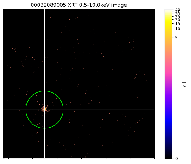
Also included in the XGA Image class is a way of overlaying the contents of a region
file. We demonstrate the simplest possible case of this here by passing the path to
the source region file we created earlier, and overlaying that one region.
It is also possible to pass a list of region objects from the
astropy-affiliated regions module.
We also demonstrate how custom ‘stretches’ (the default is a LogStretch) can be
applied to the image, by passing an astropy PowerStretch instance.
cur_im = ims[rel_obsids[-1]]

cur_im.regions = src_reg_path
cur_im.view(
    src_coord_quant,
    zoom_in=True,
    view_regions=True,
    figsize=(7, 5.5),
    stretch=PowerStretch(0.1),
)
5. Loading and fitting spectra with pyXspec#
We now wish to fit a model to the spectra that we just generated, which we hope will give us some physical insight into T Pyx’s sixth historical outburst!
In this demonstration we will use the Python interface to the XSPEC spectral fitting package, pyXspec.
Our demonstration of using pyXspec for spectral fitting will be of moderate complexity, but please note that XSPEC (and by extension pyXspec) is a very powerful tool, with a great deal of flexibility. It is not possible for us to demonstrate every aspect of pyXspec in this notebook. We encourage you to explore the pyXspec documentation, and this list of available models.
This demonstration will include fitting a multi-component model to our Swift-XRT spectra, both individually and using XSPEC’s joint-fitting functionality.
We first define path variables for the ARF and RMF files that accompany and support our spectra:
arf_temp = os.path.join(OUT_PATH, "{oi}/sw{oi}xpcw3posr.arf")
rmf_temp = os.path.join(OUT_PATH, "{oi}/swxpc0to12s6_20110101v014.rmf")
Configuring PyXspec#
Now we configure some behaviors of XSPEC/pyXspec:
The
chatterparameter is set to zero to reduce printed output during fitting (note that some XSPEC messages are still shown).We inform XSPEC of the number of cores we have available, as some XSPEC methods can be paralleled.
We tell XSPEC to use the Cash statistic for fitting (the reason we grouped our spectra earlier).
xs.Xset.chatter = 0

# XSPEC parallelisation settings
xs.Xset.parallel.leven = NUM_CORES
xs.Xset.parallel.error = NUM_CORES
xs.Xset.parallel.steppar = NUM_CORES

# Other xspec settings
xs.Plot.area = True
xs.Plot.xAxis = "keV"
xs.Plot.background = True
xs.Fit.statMethod = "cstat"
xs.Fit.query = "no"
xs.Fit.nIterations = 500
Reading spectra into pyXspec#
The first step is to load each Swift-XRT observation’s source spectrum into pyXspec, and then to point pyXspec towards the background spectrum, ARF, and RMF files.
In some cases manually specifying the locations of background, ARF, and RMF files isn’t necessary, as their paths can be embedded in a FITS header of the source spectrum file.
Every spectrum is read into a different XSPEC data group, and once loaded, we tell XSPEC to ignore any spectrum channels that are not within the 0.3-7.0 keV energy range. Choices like this are driven by the effective energy range of the instrument (XRT data below 0.3 keV are not considered trustworthy, for instance), as well as by your own analysis needs.
T Pyx is not a particularly ‘hard’ (i.e. high-energy) X-ray source, and there is very little signal above 7 keV. As such, we may get better results if we exclude those higher energies from consideration during spectral fitting. We could even move the upper energy limit down further if we found that our spectral fits were not successful.
We also explicitly exclude any spectral channels that have been marked as ‘bad’, which could have happened in the processing/generation of our X-ray data products.
# Clear out any previously loaded datasets and models
xs.AllData.clear()
xs.AllModels.clear()

# Iterating through all the ObsIDs
with tqdm(
    desc="Loading Swift-XRT spectra into pyXspec", total=len(rel_obsids)
) as onwards:
    for oi_ind, oi in enumerate(rel_obsids):
        data_grp = oi_ind + 1

        # Loading in the spectrum - making sure they all have different data groups
        xs.AllData(f"{data_grp}:{data_grp} " + grp_sp_temp.format(oi=oi))
        spec = xs.AllData(data_grp)
        spec.response = rmf_temp.format(oi=oi)
        spec.response.arf = arf_temp.format(oi=oi)
        spec.background = bsp_temp.format(oi=oi)

        spec.ignore("**-0.3 7.0-**")
        onwards.update(1)

# Ignore any channels that have been marked as 'bad'
# This CANNOT be done on a spectrum-by-spectrum basis, only after all spectra
#  have been declared
xs.AllData.ignore("bad")
Loading Swift-XRT spectra into pyXspec: 100%|██████████| 8/8 [00:02<00:00, 3.90it/s]
Fitting a model to all spectra individually#
Somewhat following the example of Chomiuk et al. (2014), we will fit a model with two additive components, a blackbody and a bremsstrahlung continuum, and an absorption component. Unlike Chomiuk et al. (2014), we do not include a Gaussian component to model the O VIII emission line.
Another model difference is that they used the tbnew plasma absorption model, whereas
we use tbabs.
Our approach is not entirely comparable to that of Chomiuk et al. (2014), as they generated week-averaged Swift-XRT spectra, not spectra from individual observations; creating combined Swift-XRT spectra is outside the scope of this demonstration, however.
By default, a model for each spectrum will be set up, with like parameters in each model ‘tied’ together; so the column density for each model will vary together, for instance, as will every other component.
Once we set reasonable parameter start values for the first model (the model assigned to the first spectrum loaded in), they will also be assigned to all other models.
We initially want to fit each spectrum completely separately, as we know that recurrent novas are, by their nature, variable with time; it would be interesting to know if the parameters of our spectral model vary over the course of these observations (around a week). As such, we ‘untie’ all the model parameters, making them completely independent:
# Set up the pyXspec model
xs.Model("tbabs*(bb+brems)")

# Setting start values for model parameters
xs.AllModels(1).setPars({1: 1, 2: 0.1, 4: 1.0, 3: 1, 5: 1})

for mod_id in range(2, len(rel_obsids) + 1):
    xs.AllModels(mod_id).untie()
To run the spectral fits, we can call the pyXspec Fit.perform() function:
xs.Fit.perform()
tbvabs Version 2.3
Cosmic absorption with grains and H2, modified from
Wilms, Allen, & McCray, 2000, ApJ 542, 914-924
Questions: Joern Wilms
joern.wilms@sternwarte.uni-erlangen.de
joern.wilms@fau.de

http://pulsar.sternwarte.uni-erlangen.de/wilms/research/tbabs/

PLEASE NOTICE:
To get the model described by the above paper
you will also have to set the abundances:
   abund wilm

Note that this routine ignores the current cross section setting
as it always HAS to use the Verner cross sections as a baseline.
We will quickly print the current values of all model parameters - though the ‘chatter’ level we specified earlier has to be temporarily relaxed in order to see the XSPEC output.
It is obvious from a glance that each model was individually fitted, as like parameters for each spectrum have different values:
xs.Xset.chatter = 10
xs.AllModels.show()
xs.Xset.chatter = 0
tbvabs Version 2.3
Cosmic absorption with grains and H2, modified from
Wilms, Allen, & McCray, 2000, ApJ 542, 914-924
Questions: Joern Wilms
joern.wilms@sternwarte.uni-erlangen.de
joern.wilms@fau.de

http://pulsar.sternwarte.uni-erlangen.de/wilms/research/tbabs/

PLEASE NOTICE:
To get the model described by the above paper
you will also have to set the abundances:
   abund wilm

Note that this routine ignores the current cross section setting
as it always HAS to use the Verner cross sections as a baseline.

Parameters defined:
========================================================================
Model TBabs<1>(bbody<2> + bremss<3>) Source No.: 1   Active/On
Model Model Component  Parameter  Unit     Value
 par  comp
                           Data group: 1
   1    1   TBabs      nH         10^22    0.109146     +/-  3.09077E-02
   2    2   bbody      kT         keV      4.98714E-02  +/-  3.88626E-03
   3    2   bbody      norm                5.89566E-03  +/-  4.23737E-03
   4    3   bremss     kT         keV      1.40213      +/-  0.269462
   5    3   bremss     norm                2.09659E-03  +/-  4.73090E-04
                           Data group: 2
   6    1   TBabs      nH         10^22    0.143126     +/-  2.13488E-02
   7    2   bbody      kT         keV      4.60205E-02  +/-  2.36086E-03
   8    2   bbody      norm                1.20866E-02  +/-  6.22295E-03
   9    3   bremss     kT         keV      1.62225      +/-  0.224638
  10    3   bremss     norm                2.61929E-03  +/-  3.62162E-04
                           Data group: 3
  11    1   TBabs      nH         10^22    8.85726E-02  +/-  2.50749E-02
  12    2   bbody      kT         keV      4.98731E-02  +/-  3.52447E-03
  13    2   bbody      norm                7.31005E-03  +/-  4.56903E-03
  14    3   bremss     kT         keV      1.58525      +/-  0.397334
  15    3   bremss     norm                2.50274E-03  +/-  5.85706E-04
                           Data group: 4
  16    1   TBabs      nH         10^22    0.142886     +/-  2.43870E-02
  17    2   bbody      kT         keV      4.30093E-02  +/-  2.65168E-03
  18    2   bbody      norm                2.80382E-02  +/-  1.83100E-02
  19    3   bremss     kT         keV      1.26972      +/-  0.183847
  20    3   bremss     norm                3.59041E-03  +/-  6.56354E-04
                           Data group: 5
  21    1   TBabs      nH         10^22    0.138989     +/-  3.79592E-02
  22    2   bbody      kT         keV      4.61061E-02  +/-  4.58728E-03
  23    2   bbody      norm                9.44736E-03  +/-  9.09029E-03
  24    3   bremss     kT         keV      0.992651     +/-  0.199343
  25    3   bremss     norm                3.67431E-03  +/-  1.11635E-03
                           Data group: 6
  26    1   TBabs      nH         10^22    0.168362     +/-  2.41903E-02
  27    2   bbody      kT         keV      4.49303E-02  +/-  2.54694E-03
  28    2   bbody      norm                1.55974E-02  +/-  9.17445E-03
  29    3   bremss     kT         keV      1.47123      +/-  0.211958
  30    3   bremss     norm                2.63791E-03  +/-  4.08549E-04
                           Data group: 7
  31    1   TBabs      nH         10^22    0.129795     +/-  4.66308E-02
  32    2   bbody      kT         keV      5.02683E-02  +/-  5.71598E-03
  33    2   bbody      norm                6.11996E-03  +/-  6.40132E-03
  34    3   bremss     kT         keV      1.91864      +/-  0.969900
  35    3   bremss     norm                1.84228E-03  +/-  6.75996E-04
                           Data group: 8
  36    1   TBabs      nH         10^22    0.165242     +/-  2.87802E-02
  37    2   bbody      kT         keV      5.02741E-02  +/-  3.20452E-03
  38    2   bbody      norm                8.12018E-03  +/-  4.92323E-03
  39    3   bremss     kT         keV      1.38293      +/-  0.239943
  40    3   bremss     norm                2.90468E-03  +/-  5.75051E-04
________________________________________________________________________
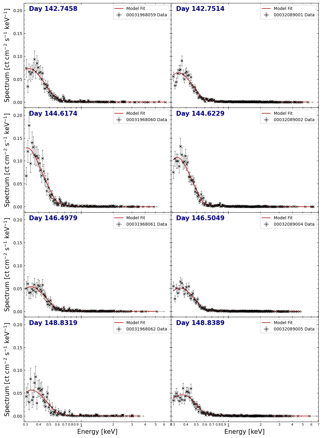
Visualizing individually fitted spectra#
Examining the spectra and their fit lines is a good way to see how well the models are representing the data, so we will make another multi-panel figure to view them all at once.
The pyXspec module has some built-in plotting capabilities, but we will instead extract the information necessary to build our own figure with matplotlib directly; it gives us much more control over the appearance of the output:
xs.Plot()

spec_plot_data = {}
fit_plot_data = {}
for oi_ind, oi in enumerate(rel_obsids):
    data_grp = oi_ind + 1

    spec_plot_data[oi] = [
        xs.Plot.x(data_grp),
        xs.Plot.xErr(data_grp),
        xs.Plot.y(data_grp),
        xs.Plot.yErr(data_grp),
    ]
    fit_plot_data[oi] = xs.Plot.model(data_grp)
Creating the figure, we can immediately see that the spectra for observations 00031968060 and 00032089002 appear to show an excess of low-energy (<0.5 keV) X-ray emission, compared to the other spectra.
Calculating uncertainties on model parameters#
Of course, being scientists, we care very much about the uncertainties of our
fitted parameter values - to get a better idea of their confidence ranges, we
can use the Fit.error() pyXspec function (which runs the XSPEC error command).
For the sake of brevity, we will focus on the errors for the column density (nH), the black body temperature, and the bremsstrahlung temperature; these are the first, second, and fourth parameters of the combined model, respectively.
When dealing with multiple data groups however, we must pass the ‘global’ parameter index to the error function. Extracting the number of parameters in a single model instance from pyXspec is simple (and of course, you could just count them), and we can use that to set up the global parameter index for every column density and temperature we constrained.
In this case we calculate the 90% confidence range for our parameters (by
passing 2.706 to error()).
Note
This step can take a few minutes to run!
# Retrieve one of the models to help get the number of parameters per model
cur_mod = xs.AllModels(1)
par_per_mod = cur_mod.nParameters

local_pars = {2: "bb_kT", 4: "br_kT"}

# Get the global parameter index for each column density, bb temperature, and
#  br temperature
err_par_ids = [
    str(par_id)
    for oi_ind in range(0, len(rel_obsids))
    for par_id in np.array(list(local_pars.keys())) + (oi_ind * par_per_mod)
]

# Run the error calculation!
xs.Fit.error("2.706 " + " ".join(err_par_ids))

# Retrieve the parameter values and uncertainties for plotting later
indiv_pars = {n: [] for n in local_pars.values()}

for mod_id in range(1, len(rel_obsids) + 1):
    cur_mod = xs.AllModels(mod_id)
    for par_id, par_name in local_pars.items():
        cur_val = cur_mod(par_id).values[0]
        cur_lims_out = cur_mod(par_id).error
        cur_err = [cur_val, cur_val - cur_lims_out[0], cur_lims_out[1] - cur_val]
        indiv_pars[par_name].append(cur_err)

        # Check the error string output by XSPEC's error command and show a warning
        #  if there might be a problem
        if cur_lims_out[2] != "FFFFFFFFF":
            warn(
                f"Error calculation for the {par_name} parameter of model {mod_id} "
                f"indicated a possible problem ({cur_lims_out[2]})",
                stacklevel=2,
            )

# Make sure the parameters are in a numpy array, easier to interact with
#  than lists of lists
indiv_pars = {n: np.array(pars) for n, pars in indiv_pars.items()}
Plotting model parameters against time#
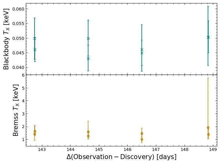
One of our stated goals was to see if the spectral properties of T Pyx varied over the course of our observations. As we have fitted models to individual spectra and calculated the uncertainties on the parameters of those models, we can now plot the parameter values against time.
Whilst we could plot the parameter values against an absolute time, we instead opt to plot against the number of days from the outburst’s discovery. Those time deltas were calculated earlier in the notebook, when we were choosing which observations to use, so we retrieve the relevant values and put them in an array:
spec_days = np.array([obs_day_from_disc_dict[oi].value for oi in rel_obsids])
We are focusing on the black body temperature and the bremsstrahlung temperature, though the normalizations of the models are also important.
It isn’t immediately obvious from the figure below whether there is a significant change in the parameters over the course of our observations; the temperature parameters could be jumping between significantly different values, which might be indicative of a model degeneracy that our individual observations are too poor to resolve.
Jointly fitting a model to all Swift-XRT spectra#
Though we found some success in the previous approach of fitting all spectra individually, it is clear that the individual observations may not have the constraining power necessary to fit our chosen model.
Chomiuk et al. (2014) also came to the conclusion that individual observations were insufficient, and decided to combine Swift-XRT observations within week-long bins. The generation of combined Swift products is beyond the scope of this demonstration, so we will attempt something similar by fitting a single model to all our Swift-XRT spectra. This should significantly increase our constraining power.
Setting up and running a joint fit#
Setting up the model for the joint is even easier than before, as we just need to declare the model, and pyXspec will automatically link all the parameter values:
# Remove all existing models
xs.AllModels.clear()

# Set up the pyXspec model
xs.Model("tbabs*(bb+brems)")

# Setting start values for model parameters
xs.AllModels(1).setPars({1: 1, 2: 0.1, 4: 1.0, 3: 1, 5: 1})
We can then run the fit, calculate uncertainties, and print the XSPEC summary of parameter values.
Once again we calculate parameter uncertainties, though this time we only have to pass two parameter-IDs, corresponding to black body temperature and bremsstrahlung temperature:
# Run the model fit
xs.Fit.perform()

# Run the error calculation
xs.Fit.error("2.706 " + " ".join([str(p_ind) for p_ind in list(local_pars.keys())]))

xs.Xset.chatter = 10
xs.AllModels.show()
xs.Xset.chatter = 0
Parameters defined:
========================================================================
Model TBabs<1>(bbody<2> + bremss<3>) Source No.: 1   Active/On
Model Model Component  Parameter  Unit     Value
 par  comp
                           Data group: 1
   1    1   TBabs      nH         10^22    0.136428     +/-  9.70306E-03
   2    2   bbody      kT         keV      4.69219E-02  +/-  1.13454E-03
   3    2   bbody      norm                1.06497E-02  +/-  2.52076E-03
   4    3   bremss     kT         keV      1.43407      +/-  9.06427E-02
   5    3   bremss     norm                2.70474E-03  +/-  1.87111E-04
                           Data group: 2
   6    1   TBabs      nH         10^22    0.136428     = p1
   7    2   bbody      kT         keV      4.69219E-02  = p2
   8    2   bbody      norm                1.06497E-02  = p3
   9    3   bremss     kT         keV      1.43407      = p4
  10    3   bremss     norm                2.70474E-03  = p5
                           Data group: 3
  11    1   TBabs      nH         10^22    0.136428     = p1
  12    2   bbody      kT         keV      4.69219E-02  = p2
  13    2   bbody      norm                1.06497E-02  = p3
  14    3   bremss     kT         keV      1.43407      = p4
  15    3   bremss     norm                2.70474E-03  = p5
                           Data group: 4
  16    1   TBabs      nH         10^22    0.136428     = p1
  17    2   bbody      kT         keV      4.69219E-02  = p2
  18    2   bbody      norm                1.06497E-02  = p3
  19    3   bremss     kT         keV      1.43407      = p4
  20    3   bremss     norm                2.70474E-03  = p5
                           Data group: 5
  21    1   TBabs      nH         10^22    0.136428     = p1
  22    2   bbody      kT         keV      4.69219E-02  = p2
  23    2   bbody      norm                1.06497E-02  = p3
  24    3   bremss     kT         keV      1.43407      = p4
  25    3   bremss     norm                2.70474E-03  = p5
                           Data group: 6
  26    1   TBabs      nH         10^22    0.136428     = p1
  27    2   bbody      kT         keV      4.69219E-02  = p2
  28    2   bbody      norm                1.06497E-02  = p3
  29    3   bremss     kT         keV      1.43407      = p4
  30    3   bremss     norm                2.70474E-03  = p5
                           Data group: 7
  31    1   TBabs      nH         10^22    0.136428     = p1
  32    2   bbody      kT         keV      4.69219E-02  = p2
  33    2   bbody      norm                1.06497E-02  = p3
  34    3   bremss     kT         keV      1.43407      = p4
  35    3   bremss     norm                2.70474E-03  = p5
                           Data group: 8
  36    1   TBabs      nH         10^22    0.136428     = p1
  37    2   bbody      kT         keV      4.69219E-02  = p2
  38    2   bbody      norm                1.06497E-02  = p3
  39    3   bremss     kT         keV      1.43407      = p4
  40    3   bremss     norm                2.70474E-03  = p5
________________________________________________________________________
Joint fit results#
Finally, we will retrieve the value and uncertainty results of the joint fit:
cur_mod = xs.AllModels(1)

for par_id, par_name in local_pars.items():
    cur_val = cur_mod(par_id).values[0]
    cur_lims_out = cur_mod(par_id).error
    cur_err = np.array([cur_val - cur_lims_out[0], cur_lims_out[1] - cur_val])

    if cur_lims_out[2] != "FFFFFFFFF":
        warn(
            f"Error calculation for the {par_name} parameter "
            f"indicated a possible problem ({cur_lims_out[2]})",
            stacklevel=2,
        )

    if par_name == "nH":
        u_str = r" $\times 10^{22}$ cm$^{-2}$"
    elif par_name == "bb_kT":
        cur_val *= 1000
        cur_err *= 1000
        u_str = " eV"
    elif par_name == "br_kT":
        u_str = " keV"

    r_str = f"{par_name} = ${cur_val:.3f}_{{-{cur_err[0]:.3f}}}^{{+{cur_err[1]:.3f}}}$"
    full_out = r_str + u_str

    display(Markdown(full_out))
bb_kT = $46.922_{-1.915}^{+1.969}$ eV
br_kT = $1.434_{-0.131}^{+0.151}$ keV
From this we can see that the temperature of the black body component is significantly lower than the bremsstrahlung temperature. This finding, and the values of the temperatures that we measure, are broadly consistent with the results for the day 142-149 period results presented by Chomiuk et al. (2014).
About this notebook#
Author: David Turner, HEASARC Staff Scientist
Author: Peter Craig, Michigan State University Research Associate
Updated On: 2025-12-23
Additional Resources#
Acknowledgements#
David Turner thanks Peter Craig (Michigan State University) for volunteering one of his favourite Swift-XRT sources for this demonstration.